【Apollo学习笔记】——规划模块TASK之PIECEWISE_JERK_SPEED_OPTIMIZER
文章目录
- TASK系列解析文章
- 前言
- PIECEWISE_JERK_SPEED_OPTIMIZER功能简介
- PIECEWISE_JERK_SPEED_OPTIMIZER相关配置
- PIECEWISE_JERK_SPEED_OPTIMIZER流程
- QP问题的标准类型定义:
- 优化变量
- 设计目标函数
- 约束条件
- 相关矩阵
- 二次项系数矩阵 H H H
- 一次项系数向量 q q q
- 设定OSQP求解参数
- Process
- 设置相关参数
- 更新STBoundary
- 更新速度边界和参考s
- 速度优化
- 输出
TASK系列解析文章
1.【Apollo学习笔记】——规划模块TASK之LANE_CHANGE_DECIDER
2.【Apollo学习笔记】——规划模块TASK之PATH_REUSE_DECIDER
3.【Apollo学习笔记】——规划模块TASK之PATH_BORROW_DECIDER
4.【Apollo学习笔记】——规划模块TASK之PATH_BOUNDS_DECIDER
5.【Apollo学习笔记】——规划模块TASK之PIECEWISE_JERK_PATH_OPTIMIZER
6.【Apollo学习笔记】——规划模块TASK之PATH_ASSESSMENT_DECIDER
7.【Apollo学习笔记】——规划模块TASK之PATH_DECIDER
8.【Apollo学习笔记】——规划模块TASK之RULE_BASED_STOP_DECIDER
9.【Apollo学习笔记】——规划模块TASK之SPEED_BOUNDS_PRIORI_DECIDER&&SPEED_BOUNDS_FINAL_DECIDER
10.【Apollo学习笔记】——规划模块TASK之SPEED_HEURISTIC_OPTIMIZER
11.【Apollo学习笔记】——规划模块TASK之SPEED_DECIDER
12.【Apollo学习笔记】——规划模块TASK之PIECEWISE_JERK_SPEED_OPTIMIZER
13.【Apollo学习笔记】——规划模块TASK之PIECEWISE_JERK_NONLINEAR_SPEED_OPTIMIZER(一)
14.【Apollo学习笔记】——规划模块TASK之PIECEWISE_JERK_NONLINEAR_SPEED_OPTIMIZER(二)
前言
在Apollo星火计划学习笔记——Apollo路径规划算法原理与实践与【Apollo学习笔记】——Planning模块讲到……Stage::Process的PlanOnReferenceLine函数会依次调用task_list中的TASK,本文将会继续以LaneFollow为例依次介绍其中的TASK部分究竟做了哪些工作。由于个人能力所限,文章可能有纰漏的地方,还请批评斧正。
在modules/planning/conf/scenario/lane_follow_config.pb.txt配置文件中,我们可以看到LaneFollow所需要执行的所有task。
stage_config: {stage_type: LANE_FOLLOW_DEFAULT_STAGEenabled: truetask_type: LANE_CHANGE_DECIDERtask_type: PATH_REUSE_DECIDERtask_type: PATH_LANE_BORROW_DECIDERtask_type: PATH_BOUNDS_DECIDERtask_type: PIECEWISE_JERK_PATH_OPTIMIZERtask_type: PATH_ASSESSMENT_DECIDERtask_type: PATH_DECIDERtask_type: RULE_BASED_STOP_DECIDERtask_type: SPEED_BOUNDS_PRIORI_DECIDERtask_type: SPEED_HEURISTIC_OPTIMIZERtask_type: SPEED_DECIDERtask_type: SPEED_BOUNDS_FINAL_DECIDERtask_type: PIECEWISE_JERK_SPEED_OPTIMIZER# task_type: PIECEWISE_JERK_NONLINEAR_SPEED_OPTIMIZERtask_type: RSS_DECIDER
本文将继续介绍LaneFollow的第13个TASK——PIECEWISE_JERK_SPEED_OPTIMIZER
PIECEWISE_JERK_SPEED_OPTIMIZER功能简介
产生平滑速度规划曲线


根据ST图的可行驶区域,优化出一条平滑的速度曲线。满足一阶导、二阶导平滑(速度加速度平滑);满足道路限速;满足车辆动力学约束。
PIECEWISE_JERK_SPEED_OPTIMIZER相关配置
modules/planning/conf/planning_config.pb.txt
default_task_config: {task_type: PIECEWISE_JERK_SPEED_OPTIMIZERpiecewise_jerk_speed_optimizer_config {acc_weight: 1.0jerk_weight: 3.0kappa_penalty_weight: 2000.0ref_s_weight: 10.0ref_v_weight: 10.0}
}
PIECEWISE_JERK_SPEED_OPTIMIZER流程
动态规划得到的轨迹还比较粗糙,需要用优化的方法对轨迹进行进一步的平滑。基于二次规划的速度规划的方法与路径规划基本一致。
原理可以参考这篇论文:
《Optimal Trajectory Generation for Autonomous Vehicles UnderCentripetal Acceleration Constraints for In-lane Driving Scenarios》
QP问题的标准类型定义:
m i n i m i z e 1 2 ⋅ x T ⋅ H ⋅ x + f T ⋅ x s . t . L B ≤ x ≤ U B A e q x = b e q A x ≤ b minimize \frac{1}{2} \cdot x^T \cdot H \cdot x + f^T \cdot x \\ s.t. LB \leq x \leq UB \\ A_{eq}x = b_{eq} \\ Ax \leq b minimize21⋅xT⋅H⋅x+fT⋅xs.t.LB≤x≤UBAeqx=beqAx≤b
优化变量

注意:速度规划的 s s s沿着轨迹的方向,路径规划的 s s s沿着参考线的方向。
 优化变量 x x x, x x x有三个部分组成:从 s 0 s_0 s0, s 1 s_1 s1, s 2 s_2 s2到 s n − 1 s_{n-1} sn−1,从 s ˙ 0 \dot s_0 s˙0, s ˙ 1 \dot s_1 s˙1, s ˙ 2 \dot s_2 s˙2到 s ˙ n − 1 \dot s_{n-1} s˙n−1,从 s ¨ 0 \ddot s_0 s¨0, s ¨ 1 \ddot s_1 s¨1, s ¨ 2 \ddot s_2 s¨2到 s ¨ n − 1 \ddot s_{n-1} s¨n−1.
x = { s 0 , s 1 , … , s n − 1 , s 0 ˙ , s 1 ˙ , … , s n − 1 ˙ , s 0 ¨ , s 1 ¨ , … , s n − 1 ¨ } x=\{s_0,s_1,\ldots,s_{n-1},\dot{s_0},\dot{s_1},\ldots,\dot{s_{n-1}},\ddot{s_0},\ddot{s_1},\ldots,\ddot{s_{n-1}}\} x={s0,s1,…,sn−1,s0˙,s1˙,…,sn−1˙,s0¨,s1¨,…,sn−1¨}
ps:三阶导的求解方式为: s ′ ′ ′ = s ′ ′ i + 1 − s ′ ′ i Δ t s^{'''}=\frac{{{{s''}_{i + 1}} - {{s''}_i}}}{{\Delta t}} s′′′=Δts′′i+1−s′′i
设计目标函数
对于目标函数的设计,我们需要明确以下目标:
- 尽可能贴合决策时制定的st曲线: ∣ s i − s i − r e f ∣ ↓ \left| {{s_i} - {s_{i - ref}}} \right| \downarrow ∣si−si−ref∣↓
- 确保舒适的体感,尽可能降低加速度/加加速度: ∣ s ¨ i + 1 ∣ ↓ \left| {{{\ddot s}_{i + 1}}} \right| \downarrow ∣s¨i+1∣↓, ∣ s ′ ′ ′ i → i + 1 ∣ ↓ \left| {{{s'''}_{i \to i + 1}}} \right| \downarrow ∣s′′′i→i+1∣↓
- 尽可能按照巡航速度行驶: ∣ s ˙ i − v r e f ∣ ↓ \left| {{{\dot s}_i} - {v_{ref}}} \right| \downarrow ∣s˙i−vref∣↓
- 在转弯时减速行驶, 曲率越大,速度越小,减小向心加速度: ∣ s ˙ i 2 κ s i ∣ ↓ \left| \dot{s}_i^2\kappa_{s_i} \right| \downarrow s˙i2κsi ↓
- 末端惩罚项,使末端 s , v , a s,v,a s,v,a趋于预期
最后会得到以下目标函数:
m i n f = ∑ i = 0 n − 1 w s ( s i − s i − r e f ) 2 + w v ( s ˙ i − v r e f ) 2 + w i s ˙ i 2 κ s i + w a s ¨ i 2 + ∑ i = 0 n − 2 w j s ′ ′ ′ i → i + 1 2 + w e n d − s ( s n − 1 − s e n d ) 2 + w e n d − d s ( s n − 1 ˙ − s e n d ˙ ) 2 + w e n d − d d s ( s n − 1 ¨ − s e n d ¨ ) 2 \begin{aligned} minf&=\sum_{i=0}^{n-1}w_s(s_i-s_{i-ref})^2+w_v(\dot{s}_i-v_{ref})^2+w_i\dot{s}_i^2\kappa_{s_i}+w_a\ddot{s}_i^2+\sum_{i=0}^{n-2}w_j{s^{'''}}_{i \to i + 1}^2\\ & +w_{end-s}(s_{n-1}-s_{end})^2+w_{end-ds}(\dot{s_{n-1}}-\dot{s_{end}})^2+w_{end-dds}(\ddot{s_{n-1}}-\ddot{s_{end}})^2 \end{aligned} minf=i=0∑n−1ws(si−si−ref)2+wv(s˙i−vref)2+wis˙i2κsi+was¨i2+i=0∑n−2wjs′′′i→i+12+wend−s(sn−1−send)2+wend−ds(sn−1˙−send˙)2+wend−dds(sn−1¨−send¨)2
w s w_s ws——位置的权重
w v w_v wv——速度的权重
w i w_i wi——曲率的权重
w a w_a wa——加速度的权重
w j w_j wj——加加速度的权重
为了统一格式,方便与代码对照,在此对目标函数进行变换:
m i n f = ∑ i = 0 n − 1 w s − r e f ( s i − s i − r e f ) 2 + w d s − r e f ( s ˙ i − s ˙ r e f ) 2 + p i s ˙ i 2 + w d d s s ¨ i 2 + ∑ i = 0 n − 2 w d d d s s ′ ′ ′ i → i + 1 2 + w e n d − s ( s n − 1 − s e n d ) 2 + w e n d − d s ( s n − 1 ˙ − s e n d ˙ ) 2 + w e n d − d d s ( s n − 1 ¨ − s e n d ¨ ) 2 \begin{aligned} minf&=\sum_{i=0}^{n-1}w_{s-ref}(s_i-s_{i-ref})^2+w_{ds-ref}(\dot{s}_i-\dot s_{ref})^2+p_i\dot{s}_i^2+w_{dds}\ddot{s}_i^2+\sum_{\color{red}i=0}^{\color{red}n-2}w_{ddds}{s^{'''}}_{i \to i + 1}^2\\ & +w_{end-s}(s_{n-1}-s_{end})^2+w_{end-ds}(\dot{s_{n-1}}-\dot{s_{end}})^2+w_{end-dds}(\ddot{s_{n-1}}-\ddot{s_{end}})^2 \end{aligned} minf=i=0∑n−1ws−ref(si−si−ref)2+wds−ref(s˙i−s˙ref)2+pis˙i2+wddss¨i2+i=0∑n−2wdddss′′′i→i+12+wend−s(sn−1−send)2+wend−ds(sn−1˙−send˙)2+wend−dds(sn−1¨−send¨)2
注: p i p_i pi代表penalty,为曲率 κ \kappa κ与曲率的权重 w i w_i wi的乘积。
接着,对目标函数按阶次整理可得:
m i n f = ∑ i = 0 n − 1 w s − r e f ( s i − s i − r e f ) 2 + w e n d − s ( s n − 1 − s e n d ) 2 + ∑ i = 0 n − 1 w d s − r e f ( s ˙ i − s ˙ r e f ) 2 + p i s ˙ i 2 + w e n d − d s ( s n − 1 ˙ − s e n d ˙ ) 2 + ∑ i = 0 n − 1 w d d s s ¨ i 2 + w e n d − d d s ( s n − 1 ¨ − s e n d ¨ ) 2 + ∑ i = 0 n − 2 w d d d s s ′ ′ ′ i → i + 1 2 \begin{aligned} minf&=\sum_{i=0}^{n-1}w_{s-ref}(s_i-s_{i-ref})^2+w_{end-s}(s_{n-1}-s_{end})^2\\ &+\sum_{i=0}^{n-1}w_{ds-ref}(\dot{s}_i-\dot s_{ref})^2+p_i\dot{s}_i^2+w_{end-ds}(\dot{s_{n-1}}-\dot{s_{end}})^2\\ &+\sum_{i=0}^{n-1}w_{dds}\ddot{s}_i^2+w_{end-dds}(\ddot{s_{n-1}}-\ddot{s_{end}})^2\\ &+\sum_{\color{red}i=0}^{\color{red}n-2}w_{ddds}{s^{'''}}_{i \to i + 1}^2 \end{aligned} minf=i=0∑n−1ws−ref(si−si−ref)2+wend−s(sn−1−send)2+i=0∑n−1wds−ref(s˙i−s˙ref)2+pis˙i2+wend−ds(sn−1˙−send˙)2+i=0∑n−1wddss¨i2+wend−dds(sn−1¨−send¨)2+i=0∑n−2wdddss′′′i→i+12
用 s ′ ′ ′ = s ′ ′ i + 1 − s ′ ′ i Δ t s^{'''}=\frac{{{{s''}_{i + 1}} - {{s''}_i}}}{{\Delta t}} s′′′=Δts′′i+1−s′′i代入目标函数,
∑ i = 0 n − 2 ( s i ′ ′ ′ ) 2 = ( s 1 ′ ′ − s 0 ′ ′ Δ t ) 2 + ( s 2 ′ ′ − s 1 ′ ′ Δ t ) 2 + ⋯ + ( s n − 2 ′ ′ − s n − 3 ′ ′ Δ t ) 2 + ( s n − 1 ′ ′ − s n − 2 ′ ′ Δ t ) 2 = ( s 0 ′ ′ ) 2 Δ t 2 + 2 ⋅ ∑ i = 1 n − 2 ( s i ′ ′ ) 2 Δ t 2 + ( s n − 1 ′ ′ ) 2 Δ t 2 − 2 ⋅ ∑ i = 0 n − 2 s i ′ ′ ⋅ s i + 1 ′ ′ Δ t 2 \begin{aligned} \sum_{\color{red}{i=0}}^{\color{red}{n-2}}(s_i^{\prime\prime\prime})^2& =\left(\frac{s_{1}^{\prime\prime}-s_{0}^{\prime\prime}}{\Delta t}\right)^2+\left(\frac{s_{2}^{\prime\prime}-s_{1}^{\prime\prime}}{\Delta t}\right)^2+\cdots+\left(\frac{s_{n-2}^{\prime\prime}-s_{n-3}^{\prime\prime}}{\Delta t}\right)^2+\left(\frac{s_{n-1}^{\prime\prime}-s_{n-2}^{\prime\prime}}{\Delta t}\right)^2 \\ &=\frac{\left(s_0^{\prime\prime}\right)^2}{\Delta t^2}+{2}\cdot\sum_{\color{red}i=1}^{\color{red}n-2}\frac{\left(s_i^{\prime\prime}\right)^2}{\Delta t^2}+\frac{\left(s_{n-1}^{\prime\prime}\right)^2}{\Delta t^2}-{2}\cdot\sum_{\color{red}i=0}^{\color{red}n-2}\frac{s_i^{\prime\prime}\cdot s_{i+1}^{\prime\prime}}{\Delta t^2} \end{aligned} i=0∑n−2(si′′′)2=(Δts1′′−s0′′)2+(Δts2′′−s1′′)2+⋯+(Δtsn−2′′−sn−3′′)2+(Δtsn−1′′−sn−2′′)2=Δt2(s0′′)2+2⋅i=1∑n−2Δt2(si′′)2+Δt2(sn−1′′)2−2⋅i=0∑n−2Δt2si′′⋅si+1′′
m i n f = ∑ i = 0 n − 1 w s − r e f ( s i − s i − r e f ) 2 + w e n d − s ( s n − 1 − s e n d ) 2 + ∑ i = 0 n − 1 w d s − r e f ( s ˙ i − s ˙ r e f ) 2 + p i s ˙ i 2 + w e n d − d s ( s n − 1 ˙ − s e n d ˙ ) 2 + ∑ i = 0 n − 1 w d d s s ¨ i 2 + w e n d − d d s ( s n − 1 ¨ − s e n d ¨ ) 2 + w d d d s [ ( s 0 ′ ′ ) 2 Δ t 2 + 2 ⋅ ∑ i = 1 n − 2 ( s i ′ ′ ) 2 Δ t 2 + ( s n − 1 ′ ′ ) 2 Δ t 2 − 2 ⋅ ∑ i = 0 n − 2 s i ′ ′ ⋅ s i + 1 ′ ′ Δ t 2 ] \begin{aligned} minf&=\sum_{i=0}^{n-1}w_{s-ref}(s_i-s_{i-ref})^2+w_{end-s}(s_{n-1}-s_{end})^2\\ &+\sum_{i=0}^{n-1}w_{ds-ref}(\dot{s}_i-\dot s_{ref})^2+p_i\dot{s}_i^2+w_{end-ds}(\dot{s_{n-1}}-\dot{s_{end}})^2\\ &+\sum_{i=0}^{n-1}w_{dds}\ddot{s}_i^2+w_{end-dds}(\ddot{s_{n-1}}-\ddot{s_{end}})^2\\ &+w_{ddds}[\frac{\left(s_0^{\prime\prime}\right)^2}{\Delta t^2}+{2}\cdot\sum_{\color{red}i=1}^{\color{red}n-2}\frac{\left(s_i^{\prime\prime}\right)^2}{\Delta t^2}+\frac{\left(s_{n-1}^{\prime\prime}\right)^2}{\Delta t^2}-{2}\cdot\sum_{\color{red}i=0}^{\color{red}n-2}\frac{s_i^{\prime\prime}\cdot s_{i+1}^{\prime\prime}}{\Delta t^2}] \end{aligned} minf=i=0∑n−1ws−ref(si−si−ref)2+wend−s(sn−1−send)2+i=0∑n−1wds−ref(s˙i−s˙ref)2+pis˙i2+wend−ds(sn−1˙−send˙)2+i=0∑n−1wddss¨i2+wend−dds(sn−1¨−send¨)2+wddds[Δt2(s0′′)2+2⋅i=1∑n−2Δt2(si′′)2+Δt2(sn−1′′)2−2⋅i=0∑n−2Δt2si′′⋅si+1′′]
约束条件
接下来谈谈约束的设计。
要满足的约束条件:
• 主车必须在道路边界内,同时不能和障碍物有碰撞 s i ∈ ( s min i , s max i ) {s_i} \in (s_{\min }^i,s_{\max }^i) si∈(smini,smaxi)• 根据当前状态,主车的横向速度/加速度/加加速度有特定运动学限制:
s i ′ ∈ ( s m i n i ′ ( t ) , s m a x i ′ ( t ) ) , s i ′ ′ ∈ ( s m i n i ′ ′ ( t ) , s m a x i ′ ′ ( t ) ) , s i ′ ′ ′ ∈ ( s m i n i ′ ′ ′ ( t ) , s m a x i ′ ′ ′ ( t ) ) s_{i}^{\prime}\in\left(s_{min}^{i}{}^{\prime}(t),s_{max}^{i}{}^{\prime}(t)\right)\text{,}s_{i}^{\prime\prime}\in\left(s_{min}^{i}{}^{\prime\prime}(t),s_{max}^{i}{}^{\prime\prime}(t)\right)\text{,}s_{i}^{\prime\prime\prime}\in\left(s_{min}^{i}{}^{\prime\prime\prime}(t),s_{max}^{i}{}^{\prime\prime\prime}(t)\right) si′∈(smini′(t),smaxi′(t)),si′′∈(smini′′(t),smaxi′′(t)),si′′′∈(smini′′′(t),smaxi′′′(t))
• 连续性约束:
s i + 1 ′ ′ = s i ′ ′ + ∫ 0 Δ t s i → i + 1 ′ ′ ′ d t = s i ′ ′ + s i → i + 1 ′ ′ ′ ∗ Δ t s i + 1 ′ = s i ′ + ∫ 0 Δ t s ′ ′ ( t ) d t = s i ′ + s i ′ ′ ∗ Δ t + 1 2 ∗ s i → i + 1 ′ ′ ′ ∗ Δ t 2 = s i ′ + 1 2 ∗ s i ′ ′ ∗ Δ t + 1 2 ∗ s i + 1 ′ ′ ∗ Δ t s i + 1 = s i + ∫ 0 Δ t s ′ ( t ) d t = s i + s i ′ ∗ Δ t + 1 2 ∗ s i ′ ′ ∗ Δ t 2 + 1 6 ∗ s i → i + 1 ′ ′ ′ ∗ Δ t 3 = s i + s i ′ ∗ Δ t + 1 3 ∗ s i ′ ′ ∗ Δ t 2 + 1 6 ∗ s i + 1 ′ ′ ∗ Δ t 2 \begin{aligned} s_{i+1}^{\prime\prime} &=s_i''+\int_0^{\Delta t}s_{i\to i+1}^{\prime\prime\prime}dt=s_i''+s_{i\to i+1}^{\prime\prime\prime}*\Delta t \\ s_{i+1}^{\prime} &=s_i^{\prime}+\int_0^{\Delta t}\boldsymbol{s''}(t)dt=s_i^{\prime}+s_i^{\prime\prime}*\Delta t+\frac12*s_{i\to i+1}^{\prime\prime\prime}*\Delta t^2 \\ &= s_i^{\prime}+\frac12*s_i^{\prime\prime}*\Delta t+\frac12*s_{i+1}^{\prime\prime}*\Delta t\\ s_{i+1} &=s_i+\int_0^{\Delta t}\boldsymbol{s'}(t)dt \\ &=s_i+s_i^{\prime}*\Delta t+\frac12*s_i^{\prime\prime}*\Delta t^2+\frac16*s_{i\to i+1}^{\prime\prime\prime}*\Delta t^3\\ &=s_i+s_i^{\prime}*\Delta t+\frac13*s_i^{\prime\prime}*\Delta t^2+\frac16*s_{i+1}^{\prime\prime}*\Delta t^2 \end{aligned} si+1′′si+1′si+1=si′′+∫0Δtsi→i+1′′′dt=si′′+si→i+1′′′∗Δt=si′+∫0Δts′′(t)dt=si′+si′′∗Δt+21∗si→i+1′′′∗Δt2=si′+21∗si′′∗Δt+21∗si+1′′∗Δt=si+∫0Δts′(t)dt=si+si′∗Δt+21∗si′′∗Δt2+61∗si→i+1′′′∗Δt3=si+si′∗Δt+31∗si′′∗Δt2+61∗si+1′′∗Δt2
• 起点约束: s 0 = s i n i t s_0=s_{init} s0=sinit, s ˙ 0 = s ˙ i n i t \dot s_0=\dot s_{init} s˙0=s˙init, s ¨ 0 = s ¨ i n i t \ddot s_0=\ddot s_{init} s¨0=s¨init满足的是起点的约束,即为实际车辆规划起点的状态。
可以看到和路径规划部分的约束条件基本一致,因此在约束矩阵 A A A部分,路径规划和速度规划矩阵一致,不用再次编写。
相关矩阵
回到代码中,PiecewiseJerkSpeedOptimizer的主流程依旧在Process中,我们暂且不关注其他细节,先关注与二次规划主体部分。
以下代码创建了一个类为PiecewiseJerkSpeedProblem的对象piecewise_jerk_problem,PiecewiseJerkSpeedProblem继承自PiecewiseJerkProblem。其中参数意义如下:
num_of_knots:表示采样点的数量。
delta_t:表示每个采样点之间的时间间隔。
init_s:表示起点位置。
// 分段加加速度速度优化算法PiecewiseJerkSpeedProblem piecewise_jerk_problem(num_of_knots, delta_t,init_s);
接着看下一段代码:
通过调用Optimize,进行二次规划问题的解决
// Solve the problemif (!piecewise_jerk_problem.Optimize()) {const std::string msg = "Piecewise jerk speed optimizer failed!";AERROR << msg;speed_data->clear();return Status(ErrorCode::PLANNING_ERROR, msg);}
Optimize这部分代码和路径规划部分一致,具体可参考【Apollo学习笔记】——规划模块TASK之PIECEWISE_JERK_PATH_OPTIMIZER
速度规划部分约束矩阵 A A A, u p p e r b o u n d upperbound upperbound, l o w e r b o u n d lowerbound lowerbound均和路径规划部分一致:
l b = [ s l b [ 0 ] ⋮ s l b [ n − 1 ] s ′ l b [ 0 ] ⋮ s ′ l b [ n − 1 ] s ′ ′ l b [ 0 ] ⋮ s ′ ′ l b [ n − 1 ] s ′ ′ ′ l b [ 0 ] ⋅ Δ t ⋮ s ′ ′ ′ l b [ n − 2 ] ⋅ Δ t 0 ⋮ 0 s i n i t s ′ i n i t s ′ ′ i n i t ] , u b = [ s u b [ 0 ] ⋮ s u b [ n − 1 ] s ′ u b [ 0 ] ⋮ s ′ u b [ n − 1 ] s ′ ′ u b [ 0 ] ⋮ s ′ ′ u b [ n − 1 ] s ′ ′ ′ u b [ 0 ] ⋅ Δ t ⋮ s ′ ′ ′ u b [ n − 2 ] ⋅ Δ t 0 ⋮ 0 s i n i t s ′ i n i t s ′ ′ i n i t ] lb = \left[ {\begin{array}{ccccccccccccccc}{{s_{lb}}[0]}\\ \vdots \\{{s_{lb}}[n - 1]}\\{{{s'}_{lb}}[0]}\\ \vdots \\{{{s'}_{lb}}[n - 1]}\\{{{s''}_{lb}}[0]}\\ \vdots \\{{{s''}_{lb}}[n - 1]}\\{{{s'''}_{lb}}[0] \cdot \Delta t}\\ \vdots \\{{{s'''}_{lb}}[n - 2] \cdot \Delta t}\\0\\ \vdots \\0\\{{s_{init}}}\\{{{s'}_{init}}}\\{{{s''}_{init}}}\end{array}} \right],ub = \left[ {\begin{array}{ccccccccccccccc}{{s_{ub}}[0]}\\ \vdots \\{{s_{ub}}[n - 1]}\\{{{s'}_{ub}}[0]}\\ \vdots \\{{{s'}_{ub}}[n - 1]}\\{{{s''}_{ub}}[0]}\\ \vdots \\{{{s''}_{ub}}[n - 1]}\\{{{s'''}_{ub}}[0] \cdot \Delta t}\\ \vdots \\{{{s'''}_{ub}}[n - 2] \cdot \Delta t}\\0\\ \vdots \\0\\{{s_{init}}}\\{{{s'}_{init}}}\\{{{s''}_{init}}}\end{array}} \right] lb= slb[0]⋮slb[n−1]s′lb[0]⋮s′lb[n−1]s′′lb[0]⋮s′′lb[n−1]s′′′lb[0]⋅Δt⋮s′′′lb[n−2]⋅Δt0⋮0sinits′inits′′init ,ub= sub[0]⋮sub[n−1]s′ub[0]⋮s′ub[n−1]s′′ub[0]⋮s′′ub[n−1]s′′′ub[0]⋅Δt⋮s′′′ub[n−2]⋅Δt0⋮0sinits′inits′′init
A = [ 1 0 ⋯ 0 0 ⋱ ⋮ ⋮ ⋱ 0 0 ⋯ 0 1 1 0 ⋯ 0 0 ⋱ ⋮ ⋮ ⋱ 0 0 ⋯ 0 1 1 0 ⋯ 0 0 ⋱ ⋮ ⋮ ⋱ 0 0 ⋯ 0 1 − 1 1 ⋱ ⋱ − 1 1 − 1 1 ⋱ ⋱ − 1 1 − Δ t 2 − Δ t 2 ⋱ ⋱ − Δ t 2 − Δ t 2 − 1 1 ⋱ ⋱ − 1 1 − Δ t ⋱ − Δ t − Δ t 2 3 − Δ t 2 6 ⋱ ⋱ − Δ t 2 3 − Δ t 2 6 1 1 1 ] A = \left[ {\begin{array}{ccccccccccccccc}{\begin{array}{ccccccccccccccc}1&0& \cdots &0\\0& \ddots &{}& \vdots \\ \vdots &{}& \ddots &0\\0& \cdots &0&1\end{array}}&{}&{}\\{}&{\begin{array}{ccccccccccccccc}1&0& \cdots &0\\0& \ddots &{}& \vdots \\ \vdots &{}& \ddots &0\\0& \cdots &0&1\end{array}}&{}\\{}&{}&{\begin{array}{ccccccccccccccc}1&0& \cdots &0\\0& \ddots &{}& \vdots \\ \vdots &{}& \ddots &0\\0& \cdots &0&1\end{array}}\\{}&{}&{\begin{array}{ccccccccccccccc}{ - 1}&1&{}&{}\\{}& \ddots & \ddots &{}\\{}&{}&{ - 1}&1\end{array}}\\{}&{\begin{array}{ccccccccccccccc}{ - 1}&1&{}&{}\\{}& \ddots & \ddots &{}\\{}&{}&{ - 1}&1\end{array}}&{\begin{array}{ccccccccccccccc}{ - \frac{{\Delta t}}{2}}&{ - \frac{{\Delta t}}{2}}&{}&{}\\{}& \ddots & \ddots &{}\\{}&{}&{ - \frac{{\Delta t}}{2}}&{ - \frac{{\Delta t}}{2}}\end{array}}\\{\begin{array}{ccccccccccccccc}{ - 1}&1&{}&{}\\{}& \ddots & \ddots &{}\\{}&{}&{ - 1}&1\end{array}}&{\begin{array}{ccccccccccccccc}{ - \Delta t}&{}&{}&{}\\{}& \ddots &{}&{}\\{}&{}&{ - \Delta t}&{}\end{array}}&{\begin{array}{ccccccccccccccc}{ - \frac{{\Delta {t^2}}}{3}}&{ - \frac{{\Delta {t^2}}}{6}}&{}&{}\\{}& \ddots & \ddots &{}\\{}&{}&{ - \frac{{\Delta {t^2}}}{3}}&{ - \frac{{\Delta {t^2}}}{6}}\end{array}}\\{\begin{array}{ccccccccccccccc}1&{}&{}&{}\\{}&{}&{}&{}\\{}&{}&{}&{}\end{array}}&{\begin{array}{ccccccccccccccc}{}&{}&{}&{}\\1&{}&{}&{}\\{}&{}&{}&{}\end{array}}&{\begin{array}{ccccccccccccccc}{}&{}&{}&{}\\{}&{}&{}&{}\\1&{}&{}&{}\end{array}}\end{array}} \right] A= 10⋮00⋱⋯⋯⋱00⋮01−11⋱⋱−11110⋮00⋱⋯⋯⋱00⋮01−11⋱⋱−11−Δt⋱−Δt110⋮00⋱⋯⋯⋱00⋮01−11⋱⋱−11−2Δt−2Δt⋱⋱−2Δt−2Δt−3Δt2−6Δt2⋱⋱−3Δt2−6Δt21
不同之处在于二次项系数矩阵 H H H与一次项系数向量 q q q
二次项系数矩阵 H H H
H = 2 ⋅ [ w s − r e f 0 ⋯ 0 0 ⋱ ⋮ ⋮ w s − r e f 0 0 ⋯ 0 w s − r e f + w e n d − s w d s − r e f + p 0 0 ⋯ 0 0 ⋱ ⋮ ⋮ w d s − r e f + p n − 2 0 0 ⋯ 0 w d s − r e f + p n − 1 + w e n d − s w d d s + w d d d s Δ t 2 0 ⋯ ⋯ 0 − 2 ⋅ w d d d s Δ t 2 w d d s + 2 ⋅ w d d d s Δ t 2 ⋮ 0 − 2 ⋅ w d d d s Δ t 2 ⋱ ⋮ ⋮ ⋱ w d d s + 2 ⋅ w d d d s Δ t 2 0 0 ⋯ 0 − 2 ⋅ w d d d s Δ t 2 w d d s + w d d d s Δ t 2 + w e n d − d d s ] H = 2 \cdot \left[ {\begin{array}{ccccccccccccccc}{\begin{array}{ccccccccccccccc}{{w_{s - ref}}}&0& \cdots &0\\0& \ddots &{}& \vdots \\ \vdots &{}&{{w_{s - ref}}}&0\\0& \cdots &0&{{w_{s - ref}} + {w_{end - s}}}\end{array}}&{}&{}\\{}&{\begin{array}{ccccccccccccccc}{{w_{ds - ref}} + {p_0}}&0& \cdots &0\\0& \ddots &{}& \vdots \\ \vdots &{}&{{w_{ds - ref}} + {p_{n - 2}}}&0\\0& \cdots &0&{{w_{ds - ref}} + {p_{n - 1}} + {w_{end - s}}}\end{array}}&{}\\{}&{}&{\begin{array}{ccccccccccccccc}{{w_{dds}} + \frac{{{w_{ddds}}}}{{\Delta {t^2}}}}&0& \cdots & \cdots &0\\{ - 2 \cdot \frac{{{w_{ddds}}}}{{\Delta {t^2}}}}&{{w_{dds}} + 2 \cdot \frac{{{w_{ddds}}}}{{\Delta {t^2}}}}&{}&{}& \vdots \\0&{ - 2 \cdot \frac{{{w_{ddds}}}}{{\Delta {t^2}}}}& \ddots &{}& \vdots \\ \vdots &{}& \ddots &{{w_{dds}} + 2 \cdot \frac{{{w_{ddds}}}}{{\Delta {t^2}}}}&0\\0& \cdots &0&{ - 2 \cdot \frac{{{w_{ddds}}}}{{\Delta {t^2}}}}&{{w_{dds}} + \frac{{{w_{ddds}}}}{{\Delta {t^2}}} + {w_{end - dds}}}\end{array}}\end{array}} \right] H=2⋅ ws−ref0⋮00⋱⋯⋯ws−ref00⋮0ws−ref+wend−swds−ref+p00⋮00⋱⋯⋯wds−ref+pn−200⋮0wds−ref+pn−1+wend−swdds+Δt2wddds−2⋅Δt2wddds0⋮00wdds+2⋅Δt2wddds−2⋅Δt2wddds⋯⋯⋱⋱0⋯wdds+2⋅Δt2wddds−2⋅Δt2wddds0⋮⋮0wdds+Δt2wddds+wend−dds
void PiecewiseJerkSpeedProblem::CalculateKernel(std::vector<c_float>* P_data,std::vector<c_int>* P_indices,std::vector<c_int>* P_indptr) {const int n = static_cast<int>(num_of_knots_);const int kNumParam = 3 * n;const int kNumValue = 4 * n - 1;std::vector<std::vector<std::pair<c_int, c_float>>> columns;columns.resize(kNumParam);int value_index = 0;// x(i)^2 * w_x_reffor (int i = 0; i < n - 1; ++i) {columns[i].emplace_back(i, weight_x_ref_ / (scale_factor_[0] * scale_factor_[0]));++value_index;}// x(n-1)^2 * (w_x_ref + w_end_x)columns[n - 1].emplace_back(n - 1, (weight_x_ref_ + weight_end_state_[0]) /(scale_factor_[0] * scale_factor_[0]));++value_index;// x(i)'^2 * (w_dx_ref + penalty_dx)for (int i = 0; i < n - 1; ++i) {columns[n + i].emplace_back(n + i,(weight_dx_ref_ + penalty_dx_[i]) /(scale_factor_[1] * scale_factor_[1]));++value_index;}// x(n-1)'^2 * (w_dx_ref + penalty_dx + w_end_dx)columns[2 * n - 1].emplace_back(2 * n - 1, (weight_dx_ref_ + penalty_dx_[n - 1] + weight_end_state_[1]) /(scale_factor_[1] * scale_factor_[1]));++value_index;auto delta_s_square = delta_s_ * delta_s_;// x(i)''^2 * (w_ddx + 2 * w_dddx / delta_s^2)columns[2 * n].emplace_back(2 * n,(weight_ddx_ + weight_dddx_ / delta_s_square) /(scale_factor_[2] * scale_factor_[2]));++value_index;for (int i = 1; i < n - 1; ++i) {columns[2 * n + i].emplace_back(2 * n + i, (weight_ddx_ + 2.0 * weight_dddx_ / delta_s_square) /(scale_factor_[2] * scale_factor_[2]));++value_index;}columns[3 * n - 1].emplace_back(3 * n - 1,(weight_ddx_ + weight_dddx_ / delta_s_square + weight_end_state_[2]) /(scale_factor_[2] * scale_factor_[2]));++value_index;// -2 * w_dddx / delta_s^2 * x(i)'' * x(i + 1)''for (int i = 0; i < n - 1; ++i) {columns[2 * n + i].emplace_back(2 * n + i + 1,-2.0 * weight_dddx_ / delta_s_square /(scale_factor_[2] * scale_factor_[2]));++value_index;}CHECK_EQ(value_index, kNumValue);int ind_p = 0;for (int i = 0; i < kNumParam; ++i) {P_indptr->push_back(ind_p);for (const auto& row_data_pair : columns[i]) {P_data->push_back(row_data_pair.second * 2.0);P_indices->push_back(row_data_pair.first);++ind_p;}}P_indptr->push_back(ind_p);
}
一次项系数向量 q q q
q = [ − 2 ⋅ w s − r e f ⋅ s 0 − r e f ⋮ − 2 ⋅ w s − r e f ⋅ s ( n − 2 ) − r e f − 2 ⋅ w s − r e f ⋅ s ( n − 1 ) − r e f − 2 ⋅ w e n d − s ⋅ s e n d − 2 ⋅ w d s − r e f ⋅ s ˙ r e f ⋮ − 2 ⋅ w d s − r e f ⋅ s ˙ r e f − 2 ⋅ w e n d − d s ⋅ s ¨ e n d − 2 ⋅ w d s − r e f ⋅ s ˙ r e f 0 ⋮ 0 − 2 ⋅ w e n d − d d s ⋅ s ¨ e n d ] q = \left[ {\begin{array}{ccccccccccccccc}{ - 2 \cdot {w_{s - ref}} \cdot {s_{0 - ref}}}\\ \vdots \\{ - 2 \cdot {w_{s - ref}} \cdot {s_{(n - 2) - ref}}}\\{ - 2 \cdot {w_{s - ref}} \cdot {s_{(n - 1) - ref}} - {\rm{2}} \cdot {w_{end - s}} \cdot {s_{end }}}\\- 2 \cdot {w_{ds - ref}} \cdot {\dot s_{ref}}\\ \vdots \\- 2 \cdot {w_{ds - ref}} \cdot {\dot s_{ref}}\\{ - {\rm{2}} \cdot {w_{end - ds}} \cdot {\ddot s_{end}}}- 2 \cdot {w_{ds - ref}} \cdot {\dot s_{ref}}\\0\\ \vdots \\0\\{ - {\rm{2}} \cdot {w_{end - dds}} \cdot {\ddot s_{end }}}\end{array}} \right] q= −2⋅ws−ref⋅s0−ref⋮−2⋅ws−ref⋅s(n−2)−ref−2⋅ws−ref⋅s(n−1)−ref−2⋅wend−s⋅send−2⋅wds−ref⋅s˙ref⋮−2⋅wds−ref⋅s˙ref−2⋅wend−ds⋅s¨end−2⋅wds−ref⋅s˙ref0⋮0−2⋅wend−dds⋅s¨end
void PiecewiseJerkSpeedProblem::CalculateOffset(std::vector<c_float>* q) {CHECK_NOTNULL(q);const int n = static_cast<int>(num_of_knots_);const int kNumParam = 3 * n;q->resize(kNumParam);for (int i = 0; i < n; ++i) {if (has_x_ref_) {q->at(i) += -2.0 * weight_x_ref_ * x_ref_[i] / scale_factor_[0];}if (has_dx_ref_) {q->at(n + i) += -2.0 * weight_dx_ref_ * dx_ref_ / scale_factor_[1];}}if (has_end_state_ref_) {q->at(n - 1) +=-2.0 * weight_end_state_[0] * end_state_ref_[0] / scale_factor_[0];q->at(2 * n - 1) +=-2.0 * weight_end_state_[1] * end_state_ref_[1] / scale_factor_[1];q->at(3 * n - 1) +=-2.0 * weight_end_state_[2] * end_state_ref_[2] / scale_factor_[2];}
}
设定OSQP求解参数
OSQPSettings* PiecewiseJerkSpeedProblem::SolverDefaultSettings() {// Define Solver default settingsOSQPSettings* settings =reinterpret_cast<OSQPSettings*>(c_malloc(sizeof(OSQPSettings)));osqp_set_default_settings(settings);settings->eps_abs = 1e-4;settings->eps_rel = 1e-4;settings->eps_prim_inf = 1e-5;settings->eps_dual_inf = 1e-5;settings->polish = true;settings->verbose = FLAGS_enable_osqp_debug;settings->scaled_termination = true;return settings;
}
Process
Process便是基于二次规划的速度优化算法的主流程了,主要包含以下步骤:
- 判断是否抵达终点,如果抵达终点,直接return。
- 检查路径是否为空
- 设置相关参数
- 更新STBoundary
- 更新速度边界和参考s
- 速度优化
- 输出
输入:
const PathData& path_data,const SpeedData& speed_data,const common::TrajectoryPoint& init_point.
输出:
得到最优的速度,信息包括 o p t _ s , o p t _ d s , o p t _ d d s opt\_s,opt\_ds,opt\_dds opt_s,opt_ds,opt_dds。在Process函数中最终结果保存到了speed_data中。
设置相关参数
StGraphData& st_graph_data = *reference_line_info_->mutable_st_graph_data();const auto& veh_param =common::VehicleConfigHelper::GetConfig().vehicle_param();// 起始点(s,v,a)std::array<double, 3> init_s = {0.0, st_graph_data.init_point().v(),st_graph_data.init_point().a()};double delta_t = 0.1;double total_length = st_graph_data.path_length();double total_time = st_graph_data.total_time_by_conf();int num_of_knots = static_cast<int>(total_time / delta_t) + 1;// 分段加加速度速度优化算法PiecewiseJerkSpeedProblem piecewise_jerk_problem(num_of_knots, delta_t,init_s);// 设置相关参数const auto& config = config_.piecewise_jerk_speed_optimizer_config();piecewise_jerk_problem.set_weight_ddx(config.acc_weight());piecewise_jerk_problem.set_weight_dddx(config.jerk_weight());piecewise_jerk_problem.set_x_bounds(0.0, total_length);piecewise_jerk_problem.set_dx_bounds(0.0, std::fmax(FLAGS_planning_upper_speed_limit,st_graph_data.init_point().v()));piecewise_jerk_problem.set_ddx_bounds(veh_param.max_deceleration(),veh_param.max_acceleration());piecewise_jerk_problem.set_dddx_bound(FLAGS_longitudinal_jerk_lower_bound,FLAGS_longitudinal_jerk_upper_bound);piecewise_jerk_problem.set_dx_ref(config.ref_v_weight(),reference_line_info_->GetCruiseSpeed());
这部分需要注意一下:
可以看到,在速度规划方面, s s s的约束为 0 ≤ s ≤ p a t h l e n g t h 0\leq s \leq pathlength 0≤s≤pathlength,此时还未考虑ST boundary; s ˙ \dot s s˙的约束为 0 ≤ s ˙ ≤ v m a x 0\leq \dot s \leq v_{max} 0≤s˙≤vmax, v m a x v_{max} vmax选出FLAGS_planning_upper_speed_limit和起始点速度之中最大的一个; s ¨ \ddot s s¨的约束为 a d e c − m a x ≤ s ¨ ≤ a a c c − m a x a_{dec-max}\leq \ddot s \leq a_{acc-max} adec−max≤s¨≤aacc−max,即在最大减速度和最大加速度范围内; s ′ ′ ′ s^{'''} s′′′的约束为 s l b ′ ′ ′ ≤ s ′ ′ ′ ≤ s u b ′ ′ ′ s^{'''}_{lb}\leq s^{'''} \leq s^{'''}_{ub} slb′′′≤s′′′≤sub′′′, j e r k jerk jerk的约束由FLAGS_longitudinal_jerk_lower_bound和FLAGS_longitudinal_jerk_upper_bound两个参数决定; s ˙ r e f \dot s_{ref} s˙ref参考速度取决于当前路径的巡航速度。
更新STBoundary
遍历每个点,根据不同障碍物类型,更新STBoundary 。
// Update STBoundarystd::vector<std::pair<double, double>> s_bounds;for (int i = 0; i < num_of_knots; ++i) {double curr_t = i * delta_t;double s_lower_bound = 0.0;double s_upper_bound = total_length;for (const STBoundary* boundary : st_graph_data.st_boundaries()) {double s_lower = 0.0;double s_upper = 0.0;if (!boundary->GetUnblockSRange(curr_t, &s_upper, &s_lower)) {continue;}switch (boundary->boundary_type()) {case STBoundary::BoundaryType::STOP:case STBoundary::BoundaryType::YIELD:s_upper_bound = std::fmin(s_upper_bound, s_upper);break;case STBoundary::BoundaryType::FOLLOW:// TODO(Hongyi): unify follow buffer on decision sides_upper_bound = std::fmin(s_upper_bound, s_upper - 8.0);break;case STBoundary::BoundaryType::OVERTAKE:s_lower_bound = std::fmax(s_lower_bound, s_lower);break;default:break;}}if (s_lower_bound > s_upper_bound) {const std::string msg ="s_lower_bound larger than s_upper_bound on STGraph";AERROR << msg;speed_data->clear();return Status(ErrorCode::PLANNING_ERROR, msg);}s_bounds.emplace_back(s_lower_bound, s_upper_bound);}piecewise_jerk_problem.set_x_bounds(std::move(s_bounds));
其中涉及到这个函数GetUnblockSRange,用途是获取未被阻塞段的s的范围。
bool STBoundary::GetUnblockSRange(const double curr_time, double* s_upper,double* s_lower) const {CHECK_NOTNULL(s_upper);CHECK_NOTNULL(s_lower);// FLAGS_speed_lon_decision_horizon: Longitudinal horizon for speed decision making (meter) 200m;*s_upper = FLAGS_speed_lon_decision_horizon;*s_lower = 0.0;// 若不在boundary的范围内,说明未被阻塞if (curr_time < min_t_ || curr_time > max_t_) {return true;}size_t left = 0;size_t right = 0;// Given time t, find a segment denoted by left and right idx, that contains the time t. // - If t is less than all or larger than all, return false.if (!GetIndexRange(lower_points_, curr_time, &left, &right)) {AERROR << "Fail to get index range.";return false;}if (curr_time > upper_points_[right].t()) {return true;}// 求出curr_time在segment中所占比例const double r =(left == right? 0.0: (curr_time - upper_points_[left].t()) /(upper_points_[right].t() - upper_points_[left].t()));// 线性插值double upper_cross_s =upper_points_[left].s() +r * (upper_points_[right].s() - upper_points_[left].s());double lower_cross_s =lower_points_[left].s() +r * (lower_points_[right].s() - lower_points_[left].s());// 根据障碍物类型,更新s_upper或s_lowerif (boundary_type_ == BoundaryType::STOP ||boundary_type_ == BoundaryType::YIELD ||boundary_type_ == BoundaryType::FOLLOW) {*s_upper = lower_cross_s;} else if (boundary_type_ == BoundaryType::OVERTAKE) {*s_lower = std::fmax(*s_lower, upper_cross_s);} else {ADEBUG << "boundary_type is not supported. boundary_type: "<< static_cast<int>(boundary_type_);return false;}return true;
}
更新速度边界和参考s
// Update SpeedBoundary and ref_sstd::vector<double> x_ref;std::vector<double> penalty_dx;std::vector<std::pair<double, double>> s_dot_bounds;const SpeedLimit& speed_limit = st_graph_data.speed_limit();for (int i = 0; i < num_of_knots; ++i) {double curr_t = i * delta_t;// get path_sSpeedPoint sp;reference_speed_data.EvaluateByTime(curr_t, &sp);const double path_s = sp.s();x_ref.emplace_back(path_s);// get curvaturePathPoint path_point = path_data.GetPathPointWithPathS(path_s);penalty_dx.push_back(std::fabs(path_point.kappa()) *config.kappa_penalty_weight());// get v_upper_boundconst double v_lower_bound = 0.0;double v_upper_bound = FLAGS_planning_upper_speed_limit;v_upper_bound = speed_limit.GetSpeedLimitByS(path_s);s_dot_bounds.emplace_back(v_lower_bound, std::fmax(v_upper_bound, 0.0));}piecewise_jerk_problem.set_x_ref(config.ref_s_weight(), std::move(x_ref));piecewise_jerk_problem.set_penalty_dx(penalty_dx);piecewise_jerk_problem.set_dx_bounds(std::move(s_dot_bounds));
速度优化
// Solve the problemif (!piecewise_jerk_problem.Optimize()) {const std::string msg = "Piecewise jerk speed optimizer failed!";AERROR << msg;speed_data->clear();return Status(ErrorCode::PLANNING_ERROR, msg);}
输出
// Extract outputconst std::vector<double>& s = piecewise_jerk_problem.opt_x();const std::vector<double>& ds = piecewise_jerk_problem.opt_dx();const std::vector<double>& dds = piecewise_jerk_problem.opt_ddx();for (int i = 0; i < num_of_knots; ++i) {ADEBUG << "For t[" << i * delta_t << "], s = " << s[i] << ", v = " << ds[i]<< ", a = " << dds[i];}speed_data->clear();speed_data->AppendSpeedPoint(s[0], 0.0, ds[0], dds[0], 0.0);for (int i = 1; i < num_of_knots; ++i) {// Avoid the very last points when already stoppedif (ds[i] <= 0.0) {break;}speed_data->AppendSpeedPoint(s[i], delta_t * i, ds[i], dds[i],(dds[i] - dds[i - 1]) / delta_t);}SpeedProfileGenerator::FillEnoughSpeedPoints(speed_data);RecordDebugInfo(*speed_data, st_graph_data.mutable_st_graph_debug());return Status::OK();
相关文章:
【Apollo学习笔记】——规划模块TASK之PIECEWISE_JERK_SPEED_OPTIMIZER
文章目录 TASK系列解析文章前言PIECEWISE_JERK_SPEED_OPTIMIZER功能简介PIECEWISE_JERK_SPEED_OPTIMIZER相关配置PIECEWISE_JERK_SPEED_OPTIMIZER流程QP问题的标准类型定义:优化变量设计目标函数约束条件相关矩阵二次项系数矩阵 H H H一次项系数向量 q q q设定OSQP求…...

CNI、CSI 和 CRI在 Docker 中的角色和作用
摘要 CNI(Container Network Interface): CNI 是用于容器网络的接口标准,它定义了容器和网络插件之间的通信协议。CNI 的主要作用是为容器创建和管理网络接口。当创建一个容器时,CNI 插件会被调用来为容器创建一个网络…...

「Docker」M1 Pro 打包docker image问题合集
运行docker 遇到 The requested images platform (linux/arm64/v8) does not match the detected host platform (linux/amd64/v4) and no specific platform was requested 说明打包的镜像没有 linux/amd64 解决方案:重新打包镜像 docker buildx build --platfor…...
Android发布依赖到 Jitpack
前言 我们在日常开发中,经常会用到第三方开源的库文件,有的来自JCenter,Maven Central,google等。但是随着JCenter的弃用,现在用的最多的还是Maven Central,google。今天我们就自己亲自发布一个依赖。 现…...
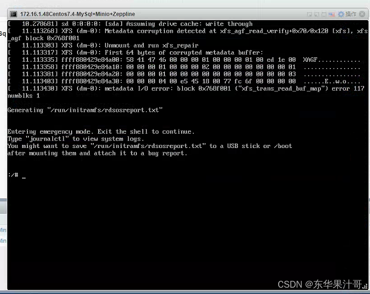
【虚拟机开不了】linux、centOS虚拟机出现entering emergency mode解决方案
按他的操作输入journalctl之后输入shiftg到日志最后查看报错发现是xfs(dm-0有问题) xfs_repair -v -L /dev/dm-0 reboot解决问题...

嘉泰实业举行“互联网金融知识社区”“安全理财风险讲座”等活动
每一次暖心的沟通都是一次公益,真诚不会因为它的渺小而被忽略;每一声问候都是一次公益,善意不会因为它的普通而被埋没。熟悉嘉泰实业的人都知道,这家企业不但擅长在金融理财领域里面呼风唤雨,同时也非常擅长在公益事业当中践行,属于企业的责任心,为更多有困难的群体带来大爱的传…...

《C++设计模式》——结构型
前言 结构模式可以让我们把很多小的东西通过结构模式组合起来成为一个打的结构,但是又不影响各自的独立性,尽可能减少各组件之间的耦合。 Adapter Class/Object(适配器) Bridge(桥接) Composite(组合) Decorator(装饰) 动态…...
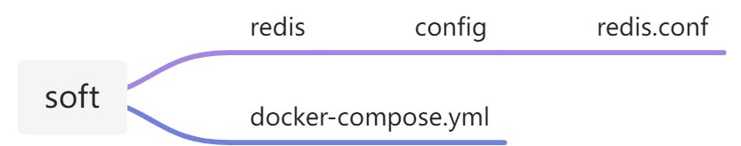
docker-compose安装redis
基于docker-compose快速安装redis 目录 一、目录结构 1、docker-compose.yml 2、redis.conf 二、连接使用 一、目录结构 1、docker-compose.yml version: 3 services:redis:image: registry.cn-hangzhou.aliyuncs.com/zhengqing/redis:6.0.8 # 镜像red…...
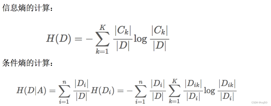
机器学习基础之《分类算法(6)—决策树》
一、决策树 1、认识决策树 决策树思想的来源非常朴素,程序设计中的条件分支结构就是if-else结构,最早的决策树就是利用这类结构分割数据的一种分类学习方法 2、一个对话的例子 想一想这个女生为什么把年龄放在最上面判断!!&…...
2023国赛数学建模C题思路模型 - 蔬菜类商品的自动定价与补货决策
# 1 赛题 在生鲜商超中,一般蔬菜类商品的保鲜期都比较短,且品相随销售时间的增加而变差, 大部分品种如当日未售出,隔日就无法再售。因此, 商超通常会根据各商品的历史销售和需 求情况每天进行补货。 由于商超销售的蔬菜…...

【Docker】Docker网络与存储(三)
前言: Docker网络与存储的作用是实现容器之间的通信和数据持久化,以便有效地部署、扩展和管理容器化应用程序。 文章目录 Docker网络桥接网络容器之间的通信 覆盖网络创建一个覆盖网络 Docker存储卷 总结 Docker网络 Docker网络是在容器之间提供通信的机…...

python面向对象的一个简单实例
#发文福利# #!/usr/bin/env python # -*- coding:utf-8 -*-students {id001: {name: serena, age: 18, address: beijing},id002: {name: fanbingbing, age: 42, address: anhui},id003: {name: kahn, age: 20, address: shanghai}}class Student:def __init__(self, xid, na…...

微信小程序通过npm引入tdesign包进行构建的时候报错
问题 在通过npm 引入 tdesign时:https://tdesign.tencent.com/miniprogram/getting-started 通过微信小程序IDE进行npm构建的时候出现:无法构建,应该怎么办? 解决方法: 1 输入: npm init -y命令 2 重新点…...

三次握手四次挥手
TCP协议是一种面向连接的、可靠的、基于字节流的运输层通信协议。它通过三次握手来建立连接,通过四次挥手来断开连接。 三次握手 所谓三次握手,是指建立一个TCP连接时,需要客户端和服务器总共发送3个报文。三次握手的目的是连接服务器指定端…...

Redis持久化、主从与哨兵架构详解
Redis持久化 RDB快照(snapshot) 在默认情况下, Redis 将内存数据库快照保存在名字为 dump.rdb 的二进制文件中。 你可以对 Redis 进行设置, 让它在“ N 秒内数据集至少有 M 个改动”这一条件被满足时, 自动保存一次数…...

SQLITE_BUSY 是指 SQLite 数据库返回的错误码,表示数据库正在被其他进程或线程使用,因此当前操作无法完成。
SQLITE_BUSY 当多个进程或线程同时尝试对同一个 SQLite 数据库进行写操作时,就可能出现 SQLITE_BUSY 错误。这是为了确保数据库的数据完整性和一致性而设计的并发控制机制。 如果你在使用 SQLite 时遇到 SQLITE_BUSY 错误,可以考虑以下解决方法&#x…...

matlab求解方程组-求解过程中限制解的取值范围
文章目录 问题背景代码my_fun.mmain.m 结果展示:不加入F(4)加入F(4) 问题背景 求解方程组的时候,对某些未知数的求解结果的取值范围有要求。例如在某些物理问题求解中,要求待求解量大于0。 代码 一共两个文件: my_fun.m main.mmy_fun.m function Fm…...

【正则表达式】正则表达式常见匹配模式
目录 常见匹配模式re.match 从字符串的起始位置匹配一个模式泛匹配匹配目标贪婪匹配非贪婪匹配匹配模式转义 re.search 扫描整个字符串并返回第一个成功的匹配re.findall 以列表形式返回全部能匹配的子串re.sub 替换字符串中每一个匹配的子串后返回替换后的字符串 re.compile 将…...

Docker搭建RK3568建模环境
推荐:Ubuntu 20.04 版本 Docker加速 # 编辑 Docker 配置文件 $ sudo vim /etc/docker/daemon.json# 加入以下配置项 {"registry-mirrors": ["https://dockerproxy.com","https://hub-mirror.c.163.com","https://mirror.baidu…...
TCP/IP基础
前言: TCP/IP协议是计算机网络领域中最基本的协议之一,它被广泛应用于互联网和局域网中,实现了不同类型、不同厂家、运行不同操作系统的计算机之间的相互通信。本文将介绍TCP/IP协议栈的层次结构、各层功能以及数据封装过程,帮助您…...

SSD用久了为啥会变慢?深入NAND Flash的‘写放大’与‘磨损均衡’,教你看懂SMART数据避坑
SSD性能下降的真相:从写放大到磨损均衡的深度解析 你是否遇到过这样的困扰——新买的SSD速度飞快,但用了一段时间后,系统响应明显变慢,开机时间延长,文件传输速度大不如前?这种现象并非偶然,而是…...
)
阿里云 ECS 部署 SpringBoot 项目完整教程(无坑可直接照着做)
需要购买阿里云服务器、学习服务器搭建的朋友看这里 👇阿里云超值折扣购买通道 :https://t.aliyun.com/U/L7DIVq 超详细服务器搭建教程:手把手教你阿里云服务器的购买及环境搭建 无论是新手入门、个人建站还是企业部署,都能一站…...
)
告别模糊:手把手教你用LAMBDA算法搞定GNSS整周模糊度(附Python代码示例)
告别模糊:手把手教你用LAMBDA算法搞定GNSS整周模糊度(附Python代码示例) 当你在开发高精度定位系统时,是否曾被整周模糊度问题困扰?这个看似简单的整数解问题,实际上影响着厘米级定位的成败。作为GNSS领域的…...

AIGlasses_for_navigation多场景落地:日常通勤、医院导诊、地铁站导航三场景实测
AIGlasses_for_navigation多场景落地:日常通勤、医院导诊、地铁站导航三场景实测 1. 引言:当导航从手机屏幕“走”到眼前 想象一下这样的场景:你走在陌生的城市街道,要去一个从未去过的咖啡馆。你不需要低头看手机地图ÿ…...

新手福音:用快马平台生成wsl安装ubuntu图文教程,轻松入门linux开发
最近在学Linux开发,发现Windows Subsystem for Linux(WSL)真是个神器,特别是搭配Ubuntu使用,既保留了Windows的便利性,又能体验原汁原味的Linux环境。不过刚开始安装配置时踩了不少坑,后来用Ins…...

3 月 21 日G-Star Gathering Day 武汉站活动精彩回顾
3 月 21 日,G-Star Gathering Day 武汉站在鄂港澳青创园顺利举办。来自 AI 与开源领域的开发者、创业者齐聚一堂,围绕 AI Agent、代码智能体、个人创业形态与真实落地场景展开分享与交流。这不仅是一场技术沙龙,更是一场关于 “AI 如何真正改…...

保姆级教程:在OpenEuler 22.03 LTS-SP4上,用cephadm搞定Ceph Pacific集群部署
在OpenEuler 22.03 LTS-SP4上部署Ceph Pacific集群的完整指南 OpenEuler作为国产操作系统的代表,凭借其高性能和安全性,正逐渐成为企业级应用的首选。而Ceph作为开源的分布式存储解决方案,以其高可靠性和可扩展性赢得了广泛认可。本文将详细介…...

AnythingtoRealCharacters2511镜像免配置部署教程:Docker+ComfyUI开箱即用方案
AnythingtoRealCharacters2511镜像免配置部署教程:DockerComfyUI开箱即用方案 想快速将动漫人物变成真实照片?这个教程教你10分钟搞定专业级动漫转真人效果,无需任何技术背景! 1. 为什么选择这个镜像? 如果你曾经尝试…...

seo规则中的内容创作有哪些注意事项
SEO规则中的内容创作有哪些注意事项 在当今互联网时代,搜索引擎优化(SEO)已成为网站流量和曝光度提升的关键手段。其中,内容创作是SEO的核心要素之一。仅仅创作大量内容并不能保证网站的高排名和高流量。要想在百度等搜索引擎上取…...
 2.0安装与验证)
保姆级教程:在Ubuntu 20.04上搞定Montreal Forced Aligner (MFA) 2.0安装与验证
保姆级教程:在Ubuntu 20.04上搞定Montreal Forced Aligner (MFA) 2.0安装与验证 语音对齐技术正在成为语音处理领域的基础工具,而Montreal Forced Aligner(MFA)作为当前最流行的开源解决方案,其2.0版本带来了显著的性…...