机器学习-数值特征
离散值处理
import pandas as pd
import numpy as np
vg_df = pd.read_csv('datasets/vgsales.csv', encoding = "ISO-8859-1")
vg_df[['Name', 'Platform', 'Year', 'Genre', 'Publisher']].iloc[1:7]
| Name | Platform | Year | Genre | Publisher | |
|---|---|---|---|---|---|
| 1 | Super Mario Bros. | NES | 1985.0 | Platform | Nintendo |
| 2 | Mario Kart Wii | Wii | 2008.0 | Racing | Nintendo |
| 3 | Wii Sports Resort | Wii | 2009.0 | Sports | Nintendo |
| 4 | Pokemon Red/Pokemon Blue | GB | 1996.0 | Role-Playing | Nintendo |
| 5 | Tetris | GB | 1989.0 | Puzzle | Nintendo |
| 6 | New Super Mario Bros. | DS | 2006.0 | Platform | Nintendo |
genres = np.unique(vg_df['Genre'])
genres
array(['Action', 'Adventure', 'Fighting', 'Misc', 'Platform', 'Puzzle','Racing', 'Role-Playing', 'Shooter', 'Simulation', 'Sports','Strategy'], dtype=object)
LabelEncoder
from sklearn.preprocessing import LabelEncodergle = LabelEncoder()
genre_labels = gle.fit_transform(vg_df['Genre'])
genre_mappings = {index: label for index, label in enumerate(gle.classes_)}
genre_mappings
{0: 'Action',1: 'Adventure',2: 'Fighting',3: 'Misc',4: 'Platform',5: 'Puzzle',6: 'Racing',7: 'Role-Playing',8: 'Shooter',9: 'Simulation',10: 'Sports',11: 'Strategy'}
vg_df['GenreLabel'] = genre_labels
vg_df[['Name', 'Platform', 'Year', 'Genre', 'GenreLabel']].iloc[1:7]
| Name | Platform | Year | Genre | GenreLabel | |
|---|---|---|---|---|---|
| 1 | Super Mario Bros. | NES | 1985.0 | Platform | 4 |
| 2 | Mario Kart Wii | Wii | 2008.0 | Racing | 6 |
| 3 | Wii Sports Resort | Wii | 2009.0 | Sports | 10 |
| 4 | Pokemon Red/Pokemon Blue | GB | 1996.0 | Role-Playing | 7 |
| 5 | Tetris | GB | 1989.0 | Puzzle | 5 |
| 6 | New Super Mario Bros. | DS | 2006.0 | Platform | 4 |
Map
poke_df = pd.read_csv('datasets/Pokemon.csv', encoding='utf-8')
poke_df = poke_df.sample(random_state=1, frac=1).reset_index(drop=True)np.unique(poke_df['Generation'])
array(['Gen 1', 'Gen 2', 'Gen 3', 'Gen 4', 'Gen 5', 'Gen 6'], dtype=object)
gen_ord_map = {'Gen 1': 1, 'Gen 2': 2, 'Gen 3': 3, 'Gen 4': 4, 'Gen 5': 5, 'Gen 6': 6}poke_df['GenerationLabel'] = poke_df['Generation'].map(gen_ord_map)
poke_df[['Name', 'Generation', 'GenerationLabel']].iloc[4:10]
| Name | Generation | GenerationLabel | |
|---|---|---|---|
| 4 | Octillery | Gen 2 | 2 |
| 5 | Helioptile | Gen 6 | 6 |
| 6 | Dialga | Gen 4 | 4 |
| 7 | DeoxysDefense Forme | Gen 3 | 3 |
| 8 | Rapidash | Gen 1 | 1 |
| 9 | Swanna | Gen 5 | 5 |
One-hot Encoding
poke_df[['Name', 'Generation', 'Legendary']].iloc[4:10]
| Name | Generation | Legendary | |
|---|---|---|---|
| 4 | Octillery | Gen 2 | False |
| 5 | Helioptile | Gen 6 | False |
| 6 | Dialga | Gen 4 | True |
| 7 | DeoxysDefense Forme | Gen 3 | True |
| 8 | Rapidash | Gen 1 | False |
| 9 | Swanna | Gen 5 | False |
from sklearn.preprocessing import OneHotEncoder, LabelEncoder# transform and map pokemon generations
gen_le = LabelEncoder()
gen_labels = gen_le.fit_transform(poke_df['Generation'])
poke_df['Gen_Label'] = gen_labels# transform and map pokemon legendary status
leg_le = LabelEncoder()
leg_labels = leg_le.fit_transform(poke_df['Legendary'])
poke_df['Lgnd_Label'] = leg_labelspoke_df_sub = poke_df[['Name', 'Generation', 'Gen_Label', 'Legendary', 'Lgnd_Label']]
poke_df_sub.iloc[4:10]
| Name | Generation | Gen_Label | Legendary | Lgnd_Label | |
|---|---|---|---|---|---|
| 4 | Octillery | Gen 2 | 1 | False | 0 |
| 5 | Helioptile | Gen 6 | 5 | False | 0 |
| 6 | Dialga | Gen 4 | 3 | True | 1 |
| 7 | DeoxysDefense Forme | Gen 3 | 2 | True | 1 |
| 8 | Rapidash | Gen 1 | 0 | False | 0 |
| 9 | Swanna | Gen 5 | 4 | False | 0 |
# encode generation labels using one-hot encoding scheme
gen_ohe = OneHotEncoder()
gen_feature_arr = gen_ohe.fit_transform(poke_df[['Gen_Label']]).toarray()
gen_feature_labels = list(gen_le.classes_)
print (gen_feature_labels)
gen_features = pd.DataFrame(gen_feature_arr, columns=gen_feature_labels)# encode legendary status labels using one-hot encoding scheme
leg_ohe = OneHotEncoder()
leg_feature_arr = leg_ohe.fit_transform(poke_df[['Lgnd_Label']]).toarray()
leg_feature_labels = ['Legendary_'+str(cls_label) for cls_label in leg_le.classes_]
print (leg_feature_labels)
leg_features = pd.DataFrame(leg_feature_arr, columns=leg_feature_labels)
['Gen 1', 'Gen 2', 'Gen 3', 'Gen 4', 'Gen 5', 'Gen 6']
['Legendary_False', 'Legendary_True']
poke_df_ohe = pd.concat([poke_df_sub, gen_features, leg_features], axis=1)
columns = sum([['Name', 'Generation', 'Gen_Label'],gen_feature_labels,['Legendary', 'Lgnd_Label'],leg_feature_labels], [])
poke_df_ohe[columns].iloc[4:10]
| Name | Generation | Gen_Label | Gen 1 | Gen 2 | Gen 3 | Gen 4 | Gen 5 | Gen 6 | Legendary | Lgnd_Label | Legendary_False | Legendary_True | |
|---|---|---|---|---|---|---|---|---|---|---|---|---|---|
| 4 | Octillery | Gen 2 | 1 | 0.0 | 1.0 | 0.0 | 0.0 | 0.0 | 0.0 | False | 0 | 1.0 | 0.0 |
| 5 | Helioptile | Gen 6 | 5 | 0.0 | 0.0 | 0.0 | 0.0 | 0.0 | 1.0 | False | 0 | 1.0 | 0.0 |
| 6 | Dialga | Gen 4 | 3 | 0.0 | 0.0 | 0.0 | 1.0 | 0.0 | 0.0 | True | 1 | 0.0 | 1.0 |
| 7 | DeoxysDefense Forme | Gen 3 | 2 | 0.0 | 0.0 | 1.0 | 0.0 | 0.0 | 0.0 | True | 1 | 0.0 | 1.0 |
| 8 | Rapidash | Gen 1 | 0 | 1.0 | 0.0 | 0.0 | 0.0 | 0.0 | 0.0 | False | 0 | 1.0 | 0.0 |
| 9 | Swanna | Gen 5 | 4 | 0.0 | 0.0 | 0.0 | 0.0 | 1.0 | 0.0 | False | 0 | 1.0 | 0.0 |
Get Dummy
gen_dummy_features = pd.get_dummies(poke_df['Generation'], drop_first=True)
pd.concat([poke_df[['Name', 'Generation']], gen_dummy_features], axis=1).iloc[4:10]
| Name | Generation | Gen 2 | Gen 3 | Gen 4 | Gen 5 | Gen 6 | |
|---|---|---|---|---|---|---|---|
| 4 | Octillery | Gen 2 | 1 | 0 | 0 | 0 | 0 |
| 5 | Helioptile | Gen 6 | 0 | 0 | 0 | 0 | 1 |
| 6 | Dialga | Gen 4 | 0 | 0 | 1 | 0 | 0 |
| 7 | DeoxysDefense Forme | Gen 3 | 0 | 1 | 0 | 0 | 0 |
| 8 | Rapidash | Gen 1 | 0 | 0 | 0 | 0 | 0 |
| 9 | Swanna | Gen 5 | 0 | 0 | 0 | 1 | 0 |
gen_onehot_features = pd.get_dummies(poke_df['Generation'])
pd.concat([poke_df[['Name', 'Generation']], gen_onehot_features], axis=1).iloc[4:10]
| Name | Generation | Gen 1 | Gen 2 | Gen 3 | Gen 4 | Gen 5 | Gen 6 | |
|---|---|---|---|---|---|---|---|---|
| 4 | Octillery | Gen 2 | 0 | 1 | 0 | 0 | 0 | 0 |
| 5 | Helioptile | Gen 6 | 0 | 0 | 0 | 0 | 0 | 1 |
| 6 | Dialga | Gen 4 | 0 | 0 | 0 | 1 | 0 | 0 |
| 7 | DeoxysDefense Forme | Gen 3 | 0 | 0 | 1 | 0 | 0 | 0 |
| 8 | Rapidash | Gen 1 | 1 | 0 | 0 | 0 | 0 | 0 |
| 9 | Swanna | Gen 5 | 0 | 0 | 0 | 0 | 1 | 0 |
import pandas as pd
import matplotlib.pyplot as plt
import matplotlib as mpl
import numpy as np
import scipy.stats as spstats%matplotlib inline
mpl.style.reload_library()
mpl.style.use('classic')
mpl.rcParams['figure.facecolor'] = (1, 1, 1, 0)
mpl.rcParams['figure.figsize'] = [6.0, 4.0]
mpl.rcParams['figure.dpi'] = 100
poke_df = pd.read_csv('datasets/Pokemon.csv', encoding='utf-8')
poke_df.head()
| # | Name | Type 1 | Type 2 | Total | HP | Attack | Defense | Sp. Atk | Sp. Def | Speed | Generation | Legendary | |
|---|---|---|---|---|---|---|---|---|---|---|---|---|---|
| 0 | 1 | Bulbasaur | Grass | Poison | 318 | 45 | 49 | 49 | 65 | 65 | 45 | Gen 1 | False |
| 1 | 2 | Ivysaur | Grass | Poison | 405 | 60 | 62 | 63 | 80 | 80 | 60 | Gen 1 | False |
| 2 | 3 | Venusaur | Grass | Poison | 525 | 80 | 82 | 83 | 100 | 100 | 80 | Gen 1 | False |
| 3 | 3 | VenusaurMega Venusaur | Grass | Poison | 625 | 80 | 100 | 123 | 122 | 120 | 80 | Gen 1 | False |
| 4 | 4 | Charmander | Fire | NaN | 309 | 39 | 52 | 43 | 60 | 50 | 65 | Gen 1 | False |
poke_df[['HP', 'Attack', 'Defense']].head()
| HP | Attack | Defense | |
|---|---|---|---|
| 0 | 45 | 49 | 49 |
| 1 | 60 | 62 | 63 |
| 2 | 80 | 82 | 83 |
| 3 | 80 | 100 | 123 |
| 4 | 39 | 52 | 43 |
poke_df[['HP', 'Attack', 'Defense']].describe()
| HP | Attack | Defense | |
|---|---|---|---|
| count | 800.000000 | 800.000000 | 800.000000 |
| mean | 69.258750 | 79.001250 | 73.842500 |
| std | 25.534669 | 32.457366 | 31.183501 |
| min | 1.000000 | 5.000000 | 5.000000 |
| 25% | 50.000000 | 55.000000 | 50.000000 |
| 50% | 65.000000 | 75.000000 | 70.000000 |
| 75% | 80.000000 | 100.000000 | 90.000000 |
| max | 255.000000 | 190.000000 | 230.000000 |
popsong_df = pd.read_csv('datasets/song_views.csv', encoding='utf-8')
popsong_df.head(10)
| user_id | song_id | title | listen_count | |
|---|---|---|---|---|
| 0 | b6b799f34a204bd928ea014c243ddad6d0be4f8f | SOBONKR12A58A7A7E0 | You're The One | 2 |
| 1 | b41ead730ac14f6b6717b9cf8859d5579f3f8d4d | SOBONKR12A58A7A7E0 | You're The One | 0 |
| 2 | 4c84359a164b161496d05282707cecbd50adbfc4 | SOBONKR12A58A7A7E0 | You're The One | 0 |
| 3 | 779b5908593756abb6ff7586177c966022668b06 | SOBONKR12A58A7A7E0 | You're The One | 0 |
| 4 | dd88ea94f605a63d9fc37a214127e3f00e85e42d | SOBONKR12A58A7A7E0 | You're The One | 0 |
| 5 | 68f0359a2f1cedb0d15c98d88017281db79f9bc6 | SOBONKR12A58A7A7E0 | You're The One | 0 |
| 6 | 116a4c95d63623a967edf2f3456c90ebbf964e6f | SOBONKR12A58A7A7E0 | You're The One | 17 |
| 7 | 45544491ccfcdc0b0803c34f201a6287ed4e30f8 | SOBONKR12A58A7A7E0 | You're The One | 0 |
| 8 | e701a24d9b6c59f5ac37ab28462ca82470e27cfb | SOBONKR12A58A7A7E0 | You're The One | 68 |
| 9 | edc8b7b1fd592a3b69c3d823a742e1a064abec95 | SOBONKR12A58A7A7E0 | You're The One | 0 |
二值特征
watched = np.array(popsong_df['listen_count'])
watched[watched >= 1] = 1
popsong_df['watched'] = watched
popsong_df.head(10)
| user_id | song_id | title | listen_count | watched | |
|---|---|---|---|---|---|
| 0 | b6b799f34a204bd928ea014c243ddad6d0be4f8f | SOBONKR12A58A7A7E0 | You're The One | 2 | 1 |
| 1 | b41ead730ac14f6b6717b9cf8859d5579f3f8d4d | SOBONKR12A58A7A7E0 | You're The One | 0 | 0 |
| 2 | 4c84359a164b161496d05282707cecbd50adbfc4 | SOBONKR12A58A7A7E0 | You're The One | 0 | 0 |
| 3 | 779b5908593756abb6ff7586177c966022668b06 | SOBONKR12A58A7A7E0 | You're The One | 0 | 0 |
| 4 | dd88ea94f605a63d9fc37a214127e3f00e85e42d | SOBONKR12A58A7A7E0 | You're The One | 0 | 0 |
| 5 | 68f0359a2f1cedb0d15c98d88017281db79f9bc6 | SOBONKR12A58A7A7E0 | You're The One | 0 | 0 |
| 6 | 116a4c95d63623a967edf2f3456c90ebbf964e6f | SOBONKR12A58A7A7E0 | You're The One | 17 | 1 |
| 7 | 45544491ccfcdc0b0803c34f201a6287ed4e30f8 | SOBONKR12A58A7A7E0 | You're The One | 0 | 0 |
| 8 | e701a24d9b6c59f5ac37ab28462ca82470e27cfb | SOBONKR12A58A7A7E0 | You're The One | 68 | 1 |
| 9 | edc8b7b1fd592a3b69c3d823a742e1a064abec95 | SOBONKR12A58A7A7E0 | You're The One | 0 | 0 |
from sklearn.preprocessing import Binarizerbn = Binarizer(threshold=0.9)
pd_watched = bn.transform([popsong_df['listen_count']])[0]
popsong_df['pd_watched'] = pd_watched
popsong_df.head(11)
| user_id | song_id | title | listen_count | watched | pd_watched | |
|---|---|---|---|---|---|---|
| 0 | b6b799f34a204bd928ea014c243ddad6d0be4f8f | SOBONKR12A58A7A7E0 | You're The One | 2 | 1 | 1 |
| 1 | b41ead730ac14f6b6717b9cf8859d5579f3f8d4d | SOBONKR12A58A7A7E0 | You're The One | 0 | 0 | 0 |
| 2 | 4c84359a164b161496d05282707cecbd50adbfc4 | SOBONKR12A58A7A7E0 | You're The One | 0 | 0 | 0 |
| 3 | 779b5908593756abb6ff7586177c966022668b06 | SOBONKR12A58A7A7E0 | You're The One | 0 | 0 | 0 |
| 4 | dd88ea94f605a63d9fc37a214127e3f00e85e42d | SOBONKR12A58A7A7E0 | You're The One | 0 | 0 | 0 |
| 5 | 68f0359a2f1cedb0d15c98d88017281db79f9bc6 | SOBONKR12A58A7A7E0 | You're The One | 0 | 0 | 0 |
| 6 | 116a4c95d63623a967edf2f3456c90ebbf964e6f | SOBONKR12A58A7A7E0 | You're The One | 17 | 1 | 1 |
| 7 | 45544491ccfcdc0b0803c34f201a6287ed4e30f8 | SOBONKR12A58A7A7E0 | You're The One | 0 | 0 | 0 |
| 8 | e701a24d9b6c59f5ac37ab28462ca82470e27cfb | SOBONKR12A58A7A7E0 | You're The One | 68 | 1 | 1 |
| 9 | edc8b7b1fd592a3b69c3d823a742e1a064abec95 | SOBONKR12A58A7A7E0 | You're The One | 0 | 0 | 0 |
| 10 | fb41d1c374d093ab643ef3bcd70eeb258d479076 | SOBONKR12A58A7A7E0 | You're The One | 1 | 1 | 1 |
多项式特征
atk_def = poke_df[['Attack', 'Defense']]
atk_def.head()
| Attack | Defense | |
|---|---|---|
| 0 | 49 | 49 |
| 1 | 62 | 63 |
| 2 | 82 | 83 |
| 3 | 100 | 123 |
| 4 | 52 | 43 |
from sklearn.preprocessing import PolynomialFeaturespf = PolynomialFeatures(degree=2, interaction_only=False, include_bias=False)
res = pf.fit_transform(atk_def)
res
array([[ 49., 49., 2401., 2401., 2401.],[ 62., 63., 3844., 3906., 3969.],[ 82., 83., 6724., 6806., 6889.],..., [ 110., 60., 12100., 6600., 3600.],[ 160., 60., 25600., 9600., 3600.],[ 110., 120., 12100., 13200., 14400.]])
intr_features = pd.DataFrame(res, columns=['Attack', 'Defense', 'Attack^2', 'Attack x Defense', 'Defense^2'])
intr_features.head(5)
| Attack | Defense | Attack^2 | Attack x Defense | Defense^2 | |
|---|---|---|---|---|---|
| 0 | 49.0 | 49.0 | 2401.0 | 2401.0 | 2401.0 |
| 1 | 62.0 | 63.0 | 3844.0 | 3906.0 | 3969.0 |
| 2 | 82.0 | 83.0 | 6724.0 | 6806.0 | 6889.0 |
| 3 | 100.0 | 123.0 | 10000.0 | 12300.0 | 15129.0 |
| 4 | 52.0 | 43.0 | 2704.0 | 2236.0 | 1849.0 |
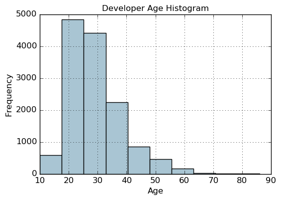
binning特征
fcc_survey_df = pd.read_csv('datasets/fcc_2016_coder_survey_subset.csv', encoding='utf-8')
fcc_survey_df[['ID.x', 'EmploymentField', 'Age', 'Income']].head()
| ID.x | EmploymentField | Age | Income | |
|---|---|---|---|---|
| 0 | cef35615d61b202f1dc794ef2746df14 | office and administrative support | 28.0 | 32000.0 |
| 1 | 323e5a113644d18185c743c241407754 | food and beverage | 22.0 | 15000.0 |
| 2 | b29a1027e5cd062e654a63764157461d | finance | 19.0 | 48000.0 |
| 3 | 04a11e4bcb573a1261eb0d9948d32637 | arts, entertainment, sports, or media | 26.0 | 43000.0 |
| 4 | 9368291c93d5d5f5c8cdb1a575e18bec | education | 20.0 | 6000.0 |
fig, ax = plt.subplots()
fcc_survey_df['Age'].hist(color='#A9C5D3')
ax.set_title('Developer Age Histogram', fontsize=12)
ax.set_xlabel('Age', fontsize=12)
ax.set_ylabel('Frequency', fontsize=12)
Text(0,0.5,'Frequency')
Binning based on rounding
Age Range: Bin
---------------0 -  9  : 0
10 - 19  : 1
20 - 29  : 2
30 - 39  : 3
40 - 49  : 4
50 - 59  : 5
60 - 69  : 6... and so on
fcc_survey_df['Age_bin_round'] = np.array(np.floor(np.array(fcc_survey_df['Age']) / 10.))
fcc_survey_df[['ID.x', 'Age', 'Age_bin_round']].iloc[1071:1076]
| ID.x | Age | Age_bin_round | |
|---|---|---|---|
| 1071 | 6a02aa4618c99fdb3e24de522a099431 | 17.0 | 1.0 |
| 1072 | f0e5e47278c5f248fe861c5f7214c07a | 38.0 | 3.0 |
| 1073 | 6e14f6d0779b7e424fa3fdd9e4bd3bf9 | 21.0 | 2.0 |
| 1074 | c2654c07dc929cdf3dad4d1aec4ffbb3 | 53.0 | 5.0 |
| 1075 | f07449fc9339b2e57703ec7886232523 | 35.0 | 3.0 |
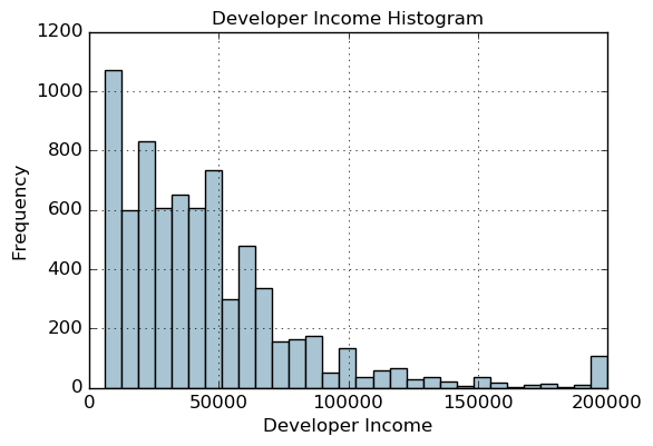
分位数切分
fcc_survey_df[['ID.x', 'Age', 'Income']].iloc[4:9]
| ID.x | Age | Income | |
|---|---|---|---|
| 4 | 9368291c93d5d5f5c8cdb1a575e18bec | 20.0 | 6000.0 |
| 5 | dd0e77eab9270e4b67c19b0d6bbf621b | 34.0 | 40000.0 |
| 6 | 7599c0aa0419b59fd11ffede98a3665d | 23.0 | 32000.0 |
| 7 | 6dff182db452487f07a47596f314bddc | 35.0 | 40000.0 |
| 8 | 9dc233f8ed1c6eb2432672ab4bb39249 | 33.0 | 80000.0 |
fig, ax = plt.subplots()
fcc_survey_df['Income'].hist(bins=30, color='#A9C5D3')
ax.set_title('Developer Income Histogram', fontsize=12)
ax.set_xlabel('Developer Income', fontsize=12)
ax.set_ylabel('Frequency', fontsize=12)
Text(0,0.5,'Frequency')
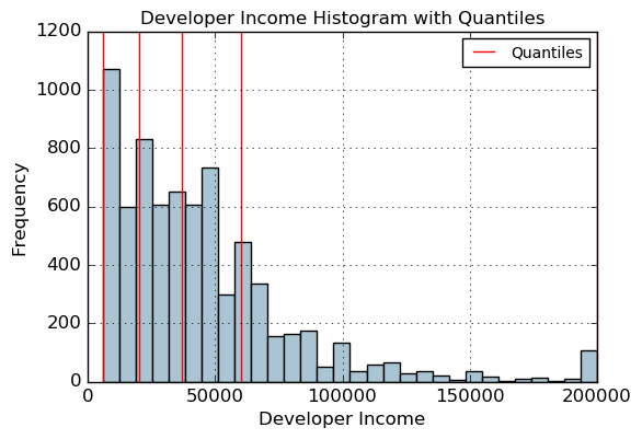
quantile_list = [0, .25, .5, .75, 1.]
quantiles = fcc_survey_df['Income'].quantile(quantile_list)
quantiles
0.00      6000.0
0.25     20000.0
0.50     37000.0
0.75     60000.0
1.00    200000.0
Name: Income, dtype: float64
fig, ax = plt.subplots()
fcc_survey_df['Income'].hist(bins=30, color='#A9C5D3')for quantile in quantiles:qvl = plt.axvline(quantile, color='r')
ax.legend([qvl], ['Quantiles'], fontsize=10)ax.set_title('Developer Income Histogram with Quantiles', fontsize=12)
ax.set_xlabel('Developer Income', fontsize=12)
ax.set_ylabel('Frequency', fontsize=12)
Text(0,0.5,'Frequency')
quantile_labels = ['0-25Q', '25-50Q', '50-75Q', '75-100Q']
fcc_survey_df['Income_quantile_range'] = pd.qcut(fcc_survey_df['Income'], q=quantile_list)
fcc_survey_df['Income_quantile_label'] = pd.qcut(fcc_survey_df['Income'], q=quantile_list, labels=quantile_labels)
fcc_survey_df[['ID.x', 'Age', 'Income', 'Income_quantile_range', 'Income_quantile_label']].iloc[4:9]
| ID.x | Age | Income | Income_quantile_range | Income_quantile_label | |
|---|---|---|---|---|---|
| 4 | 9368291c93d5d5f5c8cdb1a575e18bec | 20.0 | 6000.0 | (5999.999, 20000.0] | 0-25Q |
| 5 | dd0e77eab9270e4b67c19b0d6bbf621b | 34.0 | 40000.0 | (37000.0, 60000.0] | 50-75Q |
| 6 | 7599c0aa0419b59fd11ffede98a3665d | 23.0 | 32000.0 | (20000.0, 37000.0] | 25-50Q |
| 7 | 6dff182db452487f07a47596f314bddc | 35.0 | 40000.0 | (37000.0, 60000.0] | 50-75Q |
| 8 | 9dc233f8ed1c6eb2432672ab4bb39249 | 33.0 | 80000.0 | (60000.0, 200000.0] | 75-100Q |
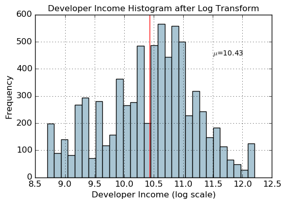
对数变换 COX-BOX
fcc_survey_df['Income_log'] = np.log((1+ fcc_survey_df['Income']))
fcc_survey_df[['ID.x', 'Age', 'Income', 'Income_log']].iloc[4:9]
| ID.x | Age | Income | Income_log | |
|---|---|---|---|---|
| 4 | 9368291c93d5d5f5c8cdb1a575e18bec | 20.0 | 6000.0 | 8.699681 |
| 5 | dd0e77eab9270e4b67c19b0d6bbf621b | 34.0 | 40000.0 | 10.596660 |
| 6 | 7599c0aa0419b59fd11ffede98a3665d | 23.0 | 32000.0 | 10.373522 |
| 7 | 6dff182db452487f07a47596f314bddc | 35.0 | 40000.0 | 10.596660 |
| 8 | 9dc233f8ed1c6eb2432672ab4bb39249 | 33.0 | 80000.0 | 11.289794 |
income_log_mean = np.round(np.mean(fcc_survey_df['Income_log']), 2)fig, ax = plt.subplots()
fcc_survey_df['Income_log'].hist(bins=30, color='#A9C5D3')
plt.axvline(income_log_mean, color='r')
ax.set_title('Developer Income Histogram after Log Transform', fontsize=12)
ax.set_xlabel('Developer Income (log scale)', fontsize=12)
ax.set_ylabel('Frequency', fontsize=12)
ax.text(11.5, 450, r'$\mu$='+str(income_log_mean), fontsize=10)
Text(11.5,450,'$\\mu$=10.43')
日期相关特征
import datetime
import numpy as np
import pandas as pd
from dateutil.parser import parse
import pytz
time_stamps = ['2015-03-08 10:30:00.360000+00:00', '2017-07-13 15:45:05.755000-07:00','2012-01-20 22:30:00.254000+05:30', '2016-12-25 00:30:00.000000+10:00']
df = pd.DataFrame(time_stamps, columns=['Time'])
df
| Time | |
|---|---|
| 0 | 2015-03-08 10:30:00.360000+00:00 |
| 1 | 2017-07-13 15:45:05.755000-07:00 |
| 2 | 2012-01-20 22:30:00.254000+05:30 |
| 3 | 2016-12-25 00:30:00.000000+10:00 |
ts_objs = np.array([pd.Timestamp(item) for item in np.array(df.Time)])
df['TS_obj'] = ts_objs
ts_objs
array([Timestamp('2015-03-08 10:30:00.360000+0000', tz='UTC'),Timestamp('2017-07-13 15:45:05.755000-0700', tz='pytz.FixedOffset(-420)'),Timestamp('2012-01-20 22:30:00.254000+0530', tz='pytz.FixedOffset(330)'),Timestamp('2016-12-25 00:30:00+1000', tz='pytz.FixedOffset(600)')], dtype=object)
df['Year'] = df['TS_obj'].apply(lambda d: d.year)
df['Month'] = df['TS_obj'].apply(lambda d: d.month)
df['Day'] = df['TS_obj'].apply(lambda d: d.day)
df['DayOfWeek'] = df['TS_obj'].apply(lambda d: d.dayofweek)
df['DayName'] = df['TS_obj'].apply(lambda d: d.weekday_name)
df['DayOfYear'] = df['TS_obj'].apply(lambda d: d.dayofyear)
df['WeekOfYear'] = df['TS_obj'].apply(lambda d: d.weekofyear)
df['Quarter'] = df['TS_obj'].apply(lambda d: d.quarter)df[['Time', 'Year', 'Month', 'Day', 'Quarter', 'DayOfWeek', 'DayName', 'DayOfYear', 'WeekOfYear']]
| Time | Year | Month | Day | Quarter | DayOfWeek | DayName | DayOfYear | WeekOfYear | |
|---|---|---|---|---|---|---|---|---|---|
| 0 | 2015-03-08 10:30:00.360000+00:00 | 2015 | 3 | 8 | 1 | 6 | Sunday | 67 | 10 |
| 1 | 2017-07-13 15:45:05.755000-07:00 | 2017 | 7 | 13 | 3 | 3 | Thursday | 194 | 28 |
| 2 | 2012-01-20 22:30:00.254000+05:30 | 2012 | 1 | 20 | 1 | 4 | Friday | 20 | 3 |
| 3 | 2016-12-25 00:30:00.000000+10:00 | 2016 | 12 | 25 | 4 | 6 | Saturday | 360 | 51 |
时间相关特征
df['Hour'] = df['TS_obj'].apply(lambda d: d.hour)
df['Minute'] = df['TS_obj'].apply(lambda d: d.minute)
df['Second'] = df['TS_obj'].apply(lambda d: d.second)
df['MUsecond'] = df['TS_obj'].apply(lambda d: d.microsecond)   #毫秒
df['UTC_offset'] = df['TS_obj'].apply(lambda d: d.utcoffset()) #UTC时间位移df[['Time', 'Hour', 'Minute', 'Second', 'MUsecond', 'UTC_offset']]
| Time | Hour | Minute | Second | MUsecond | UTC_offset | |
|---|---|---|---|---|---|---|
| 0 | 2015-03-08 10:30:00.360000+00:00 | 10 | 30 | 0 | 360000 | 00:00:00 |
| 1 | 2017-07-13 15:45:05.755000-07:00 | 15 | 45 | 5 | 755000 | -1 days +17:00:00 |
| 2 | 2012-01-20 22:30:00.254000+05:30 | 22 | 30 | 0 | 254000 | 05:30:00 |
| 3 | 2016-12-25 00:30:00.000000+10:00 | 0 | 30 | 0 | 0 | 10:00:00 |
按照早晚切分时间
hour_bins = [-1, 5, 11, 16, 21, 23]
bin_names = ['Late Night', 'Morning', 'Afternoon', 'Evening', 'Night']
df['TimeOfDayBin'] = pd.cut(df['Hour'], bins=hour_bins, labels=bin_names)
df[['Time', 'Hour', 'TimeOfDayBin']]
| Time | Hour | TimeOfDayBin | |
|---|---|---|---|
| 0 | 2015-03-08 10:30:00.360000+00:00 | 10 | Morning |
| 1 | 2017-07-13 15:45:05.755000-07:00 | 15 | Afternoon |
| 2 | 2012-01-20 22:30:00.254000+05:30 | 22 | Night |
| 3 | 2016-12-25 00:30:00.000000+10:00 | 0 | Late Night |
相关文章:
机器学习-数值特征
离散值处理 import pandas as pd import numpy as npvg_df pd.read_csv(datasets/vgsales.csv, encoding "ISO-8859-1") vg_df[[Name, Platform, Year, Genre, Publisher]].iloc[1:7]NamePlatformYearGenrePublisher1Super Mario Bros.NES1985.0PlatformNintendo2…...

Rocky(centos)安装nginx并设置开机自启
一、安装nginx 1、安装依赖 yum install -y gcc-c pcre pcre-devel zlib zlib-devel openssl openssl-devel 2、去官网下载最新的稳定版nginx nginx: downloadhttp://nginx.org/en/download.html 3、将下载后的nginx上传至/usr/local下 或者执行 #2023-10-8更新 cd /usr/…...
Android约束布局ConstraintLayout的Guideline,CardView
Android约束布局ConstraintLayout的Guideline,CardView <?xml version"1.0" encoding"utf-8"?> <androidx.constraintlayout.widget.ConstraintLayout xmlns:android"http://schemas.android.com/apk/res/android"xmlns:a…...
)
LVGL8.3.6 Flex(弹性布局)
使用lv_obj_set_flex_flow(obj, flex_flow)函数 横向拖动 LV_FLEX_FLOW_ROW 将子元素排成一排而不包裹 LV_FLEX_FLOW_ROW_WRAP 将孩子排成一排并包裹起来 LV_FLEX_FLOW_ROW_REVERSE 将子元素排成一行而不换行,但顺序相反 LV_FLEX_FLOW_ROW_WRAP_REVERSE 将子元素…...
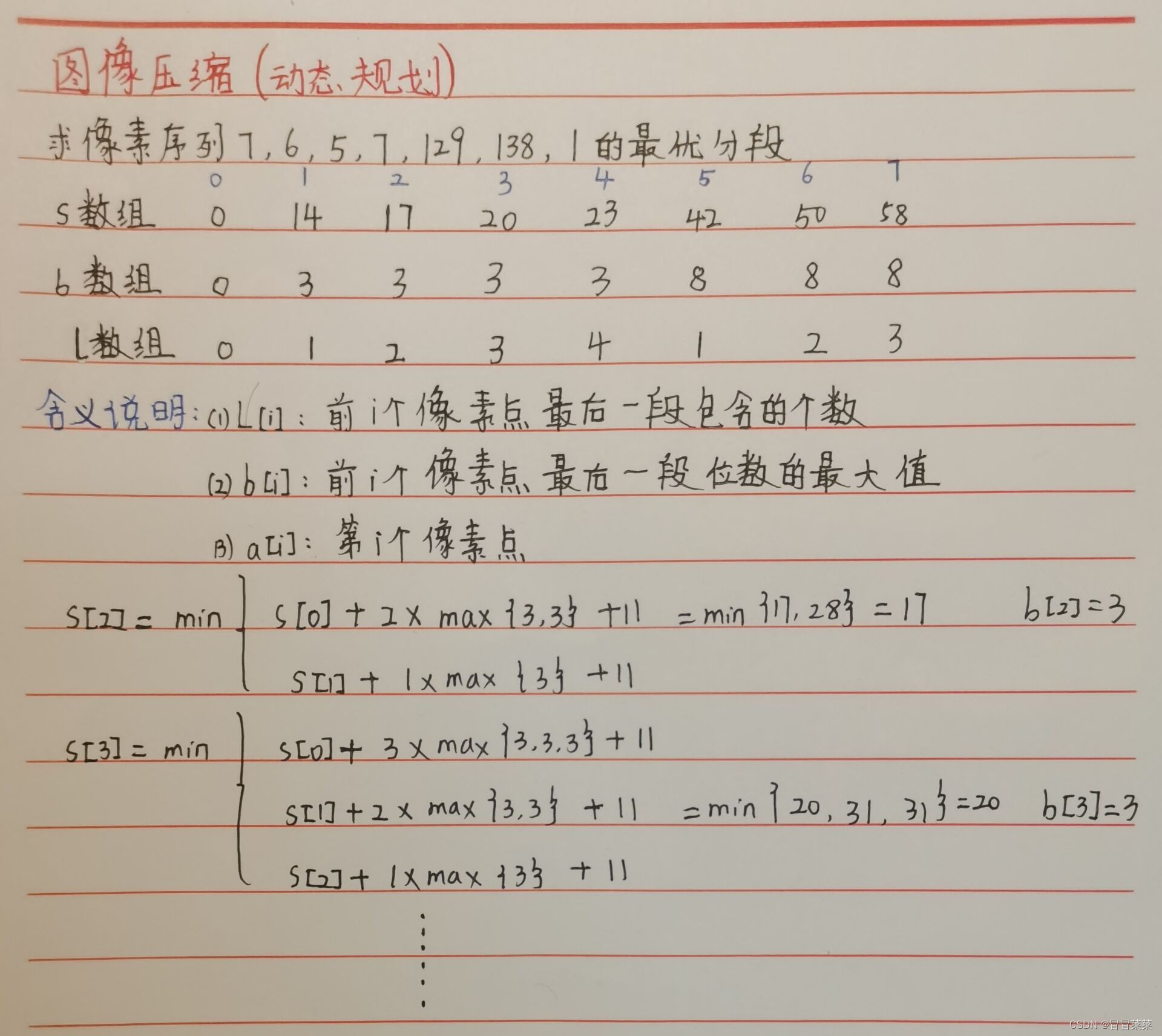
计算机算法分析与设计(8)---图像压缩动态规划算法(含C++)代码
文章目录 一、知识概述1.1 问题描述1.2 算法思想1.3 算法设计1.4 例题分析 二、代码 一、知识概述 1.1 问题描述 1. 一幅图像的由很多个像素点构成,像素点越多分辨率越高,像素的灰度值范围为0~255,也就是需要8bit来存储一个像素的灰度值信息…...
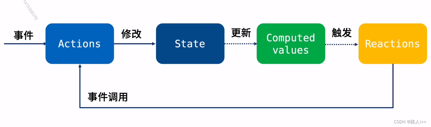
React 状态管理 - Mobx 入门(上)
Mobx是另一款优秀的状态管理方案 【让我们未来多一种状态管理选型】 响应式状态管理工具 扩展学习资料 名称 链接 备注 mobx 文档 1. MobX 介绍 MobX 中文文档 mobx https://medium.com/Zwenza/how-to-persist-your-mobx-state-4b48b3834a41 英文 Mobx核心概念 M…...
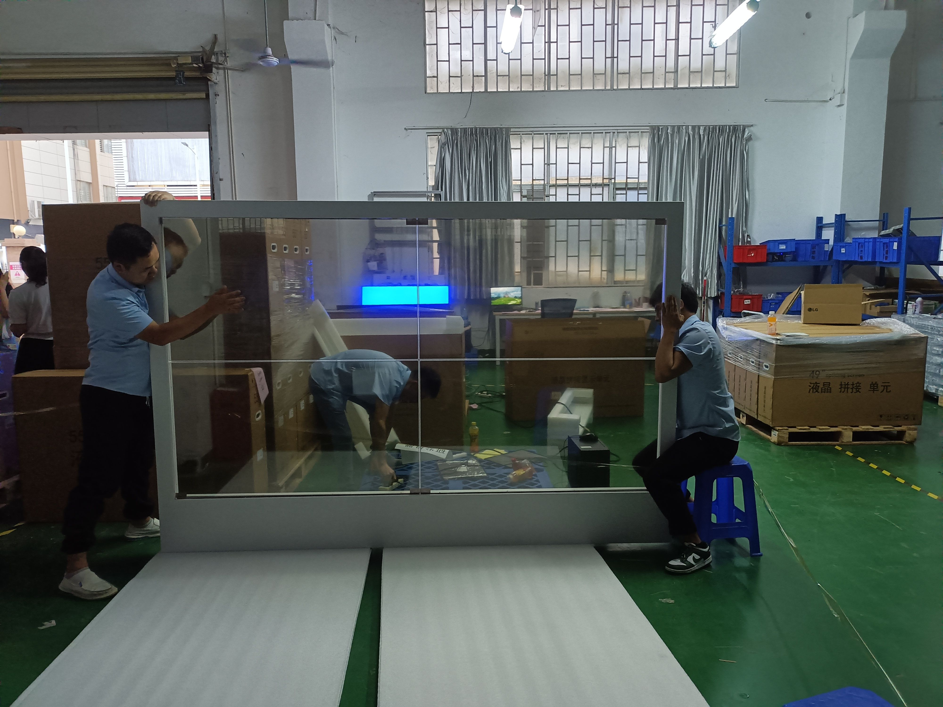
OLED透明屏技术在智能手机、汽车和广告领域的市场前景
OLED透明屏技术作为一种新型的显示技术,具有高透明度、触摸和手势交互、高画质和图像显示效果等优势,引起了广泛的关注。 随着智能手机、汽车和广告等行业的快速发展,OLED透明屏技术也在这些领域得到了广泛的应用。 本文将介绍OLED透明屏技…...

考研是为了逃避找工作的压力吗?
如果逃避眼前的现实, 越是逃就越是会陷入痛苦的境地,要有面对问题的勇气,渡过这个困境的话,应该就能一点点地解决问题。 众所周知,考研初试在大四上学期的十二月份,通常最晚的开始准备时间是大三暑假&…...

广州华锐互动:VR动物解剖实验室带来哪些便利?
随着科技的不断发展,我们的教育方式也在逐步变化和进步。其中,虚拟现实(VR)技术的应用为我们提供了一种全新的学习方式。尤其是在动物解剖实验中,VR技术不仅能够增强学习的趣味性,还能够提高学习效率和准确性。 由广州华锐互动开发…...

Uniapp 婚庆服务全套模板前端
包含 首页、社区、关于、我的、预约、订购、选购、话题、主题、收货地址、购物车、系统通知、会员卡、优惠券、积分、储值金、订单信息、积分、充值、礼品、首饰等 请观看 图片参观 开源,下载即可 链接:婚庆服务全套模板前端 - DCloud 插件市场 问题反…...
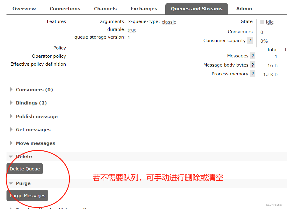
RabbitMQ-网页使用消息队列
1.使用消息队列 几种模式 从最简单的开始 添加完新的虚拟机可以看到,当前admin用户的主机访问权限中新增的刚添加的环境 1.1查看交换机 交换机列表中自动新增了刚创建好的虚拟主机相关的预设交换机。一共7个。前面两个 direct类型的交换机,一个是…...
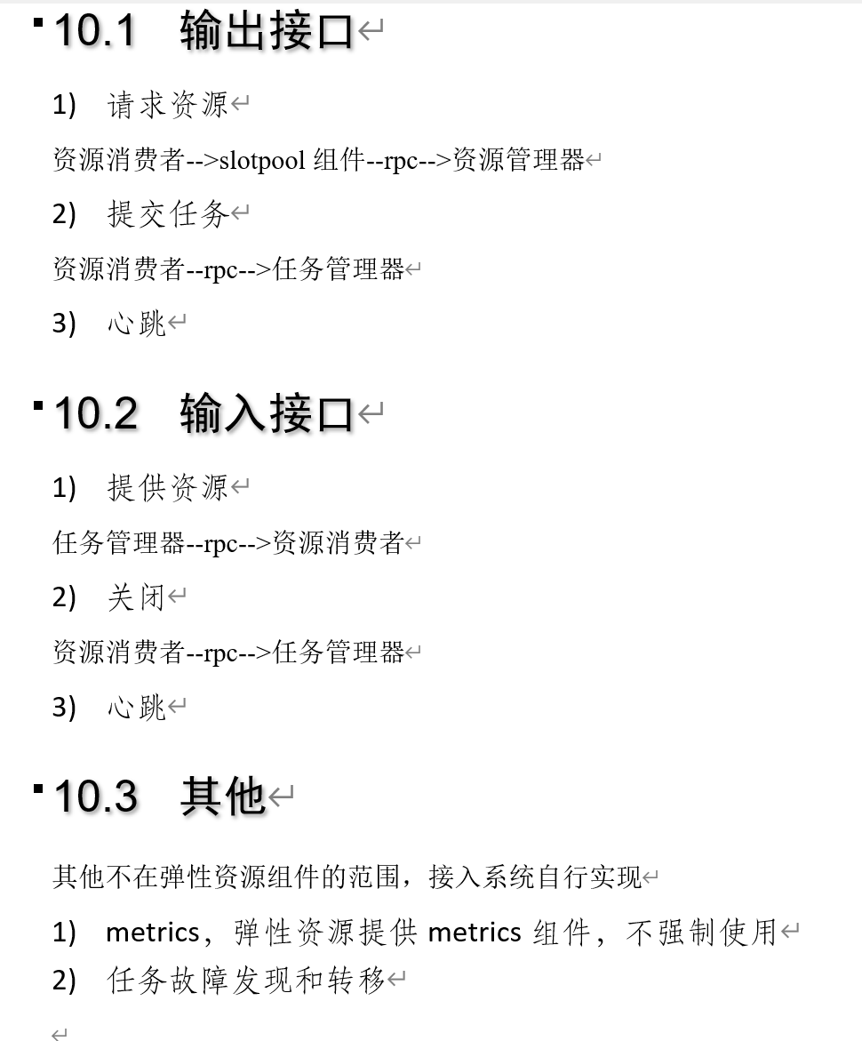
弹性资源组件elastic-resource设计(四)-任务管理器和资源消费者规范
简介 弹性资源组件提供动态资源能力,是分布式系统关键基础设施,分布式datax,分布式索引,事件引擎都需要集群和资源的弹性资源能力,提高伸缩性和作业处理能力。 本文介绍弹性资源组件的设计,包括架构设计和详…...
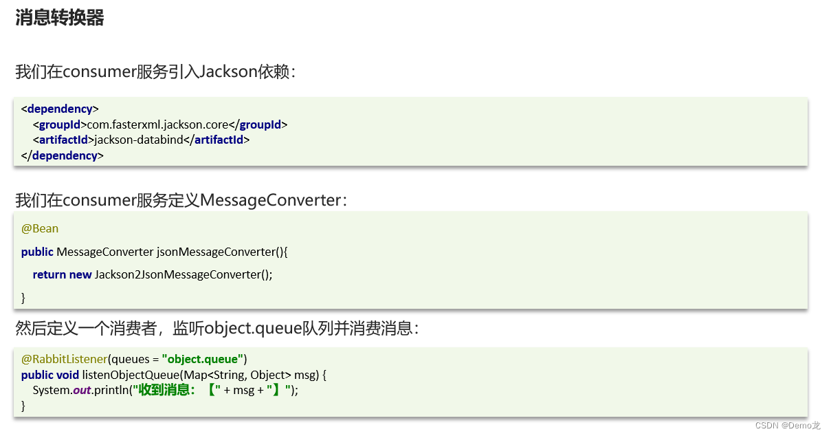
【Java】微服务——RabbitMQ消息队列(SpringAMQP实现五种消息模型)
目录 1.初识MQ1.1.同步和异步通讯1.1.1.同步通讯1.1.2.异步通讯 1.2.技术对比: 2.快速入门2.1.RabbitMQ消息模型2.4.1.publisher实现2.4.2.consumer实现 2.5.总结 3.SpringAMQP3.1.Basic Queue 简单队列模型3.1.1.消息发送3.1.2.消息接收3.1.3.测试 3.2.WorkQueue3.…...
实践例子)
react高阶成分(HOC)实践例子
以下是一个使用React函数式组件的高阶组件示例,它用于添加身份验证功能: import React, { useState, useEffect } from react;// 定义一个高阶组件,它接受一个组件作为输入,并返回一个新的包装组件 const withAuthentication (W…...
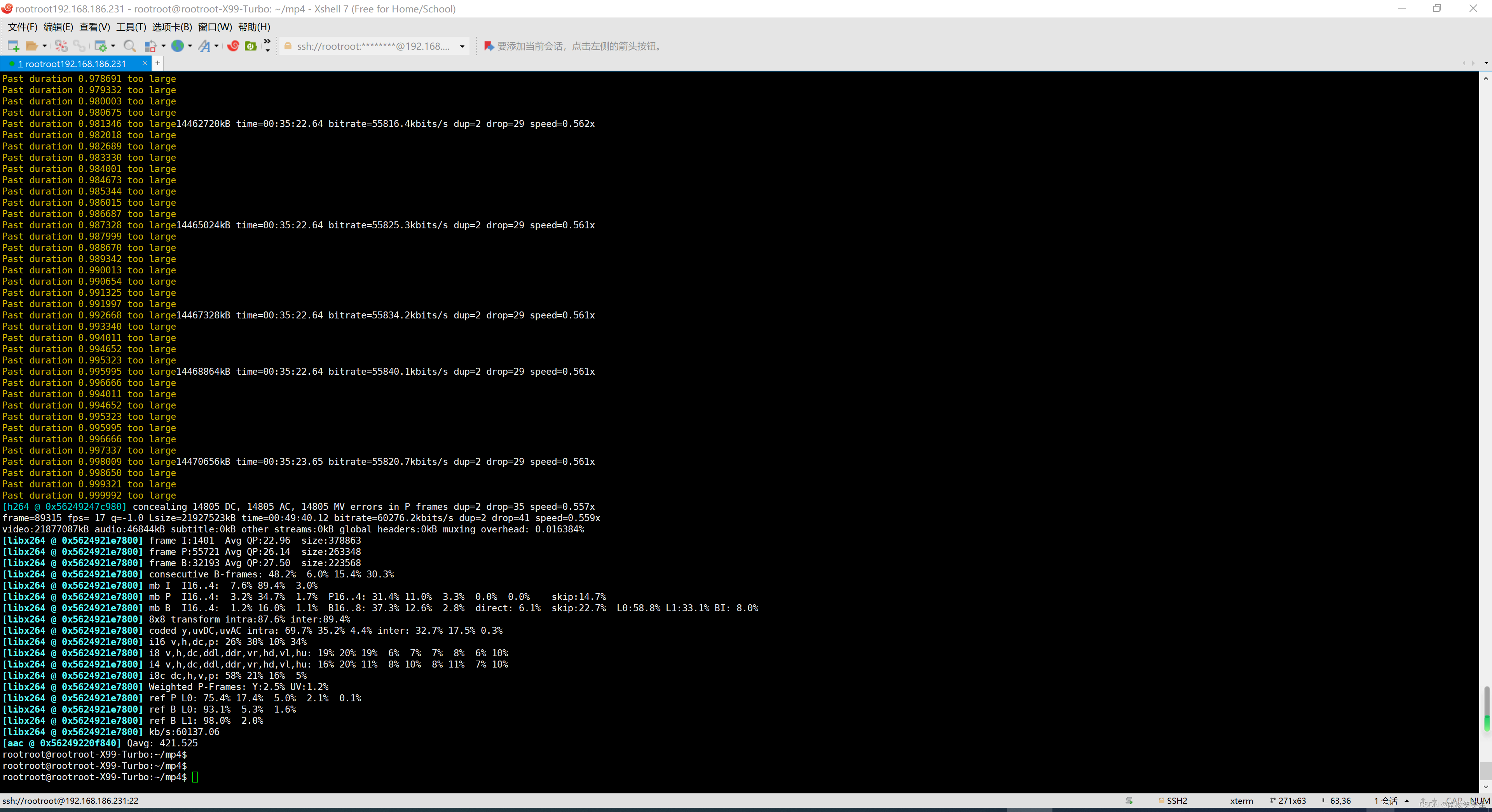
20231005使用ffmpeg旋转MP4视频
20231005使用ffmpeg旋转MP4视频 2023/10/5 12:21 百度搜搜:ffmpeg 旋转90度 https://zhuanlan.zhihu.com/p/637790915 【FFmpeg实战】FFMPEG常用命令行 https://blog.csdn.net/weixin_37515325/article/details/127817057 FFMPEG常用命令行 5.视频旋转 顺时针旋转…...
MySQL-锁
MySQL的锁机制 1.共享锁(Shared Lock)和排他锁(Exclusive Lock) 事务不能同时具有行共享锁和排他锁,如果事务想要获取排他锁,前提是行没有共享锁和排他锁。而共享锁,只要行没有排他锁都能获取到。 手动开启共享锁/排他锁: -- 对…...

ES6中变量解构赋值
数组的解构赋值 ES6规定以一定模式从数组、对象中提取值,然后给变量赋值叫做解构。 本质上就是一种匹配模式,等号两边模式相同,左边的变量就能对应的值。 假如解构不成功会赋值为undefined。 不需要匹配的位置可以置空 let [ a, b, c] …...
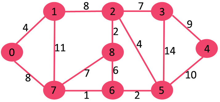
Dijkstra 邻接表表示算法 | 贪心算法实现--附C++/JAVA实现源码
以下是详细步骤。 创建大小为 V 的最小堆,其中 V 是给定图中的顶点数。最小堆的每个节点包含顶点编号和顶点的距离值。 以源顶点为根初始化最小堆(分配给源顶点的距离值为0)。分配给所有其他顶点的距离值为 INF(无限)。 当最小堆不为空时,执行以下操作: 从最小堆中提取…...

从城市吉祥物进化到虚拟人IP需要哪些步骤?
在2023年成都全国科普日主场活动中,推出了全国首个科普数字形象大使“科普熊猫”,科普熊猫作为成都科普吉祥物,是如何进化为虚拟人IP,通过动作捕捉、AR等技术,活灵活现地出现在大众眼前的? 以广州虚拟动力虚…...

认识SQLServer
深入认识SQL Server:从基础到高级的数据库管理 在当今数字时代,数据是企业成功的关键。为了存储、管理和分析数据,数据库管理系统(DBMS)变得至关重要。其中,Microsoft SQL Server是一款备受欢迎的关系型数据…...
练习(含atoi的模拟实现,自定义类型等练习)
一、结构体大小的计算及位段 (结构体大小计算及位段 详解请看:自定义类型:结构体进阶-CSDN博客) 1.在32位系统环境,编译选项为4字节对齐,那么sizeof(A)和sizeof(B)是多少? #pragma pack(4)st…...
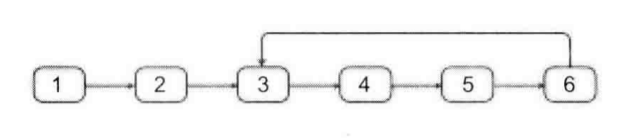
剑指offer20_链表中环的入口节点
链表中环的入口节点 给定一个链表,若其中包含环,则输出环的入口节点。 若其中不包含环,则输出null。 数据范围 节点 val 值取值范围 [ 1 , 1000 ] [1,1000] [1,1000]。 节点 val 值各不相同。 链表长度 [ 0 , 500 ] [0,500] [0,500]。 …...

ESP32 I2S音频总线学习笔记(四): INMP441采集音频并实时播放
简介 前面两期文章我们介绍了I2S的读取和写入,一个是通过INMP441麦克风模块采集音频,一个是通过PCM5102A模块播放音频,那如果我们将两者结合起来,将麦克风采集到的音频通过PCM5102A播放,是不是就可以做一个扩音器了呢…...

HTML前端开发:JavaScript 常用事件详解
作为前端开发的核心,JavaScript 事件是用户与网页交互的基础。以下是常见事件的详细说明和用法示例: 1. onclick - 点击事件 当元素被单击时触发(左键点击) button.onclick function() {alert("按钮被点击了!&…...

CRMEB 框架中 PHP 上传扩展开发:涵盖本地上传及阿里云 OSS、腾讯云 COS、七牛云
目前已有本地上传、阿里云OSS上传、腾讯云COS上传、七牛云上传扩展 扩展入口文件 文件目录 crmeb\services\upload\Upload.php namespace crmeb\services\upload;use crmeb\basic\BaseManager; use think\facade\Config;/*** Class Upload* package crmeb\services\upload* …...
第 86 场周赛:矩阵中的幻方、钥匙和房间、将数组拆分成斐波那契序列、猜猜这个单词
Q1、[中等] 矩阵中的幻方 1、题目描述 3 x 3 的幻方是一个填充有 从 1 到 9 的不同数字的 3 x 3 矩阵,其中每行,每列以及两条对角线上的各数之和都相等。 给定一个由整数组成的row x col 的 grid,其中有多少个 3 3 的 “幻方” 子矩阵&am…...
初探Service服务发现机制
1.Service简介 Service是将运行在一组Pod上的应用程序发布为网络服务的抽象方法。 主要功能:服务发现和负载均衡。 Service类型的包括ClusterIP类型、NodePort类型、LoadBalancer类型、ExternalName类型 2.Endpoints简介 Endpoints是一种Kubernetes资源…...

适应性Java用于现代 API:REST、GraphQL 和事件驱动
在快速发展的软件开发领域,REST、GraphQL 和事件驱动架构等新的 API 标准对于构建可扩展、高效的系统至关重要。Java 在现代 API 方面以其在企业应用中的稳定性而闻名,不断适应这些现代范式的需求。随着不断发展的生态系统,Java 在现代 API 方…...

【安全篇】金刚不坏之身:整合 Spring Security + JWT 实现无状态认证与授权
摘要 本文是《Spring Boot 实战派》系列的第四篇。我们将直面所有 Web 应用都无法回避的核心问题:安全。文章将详细阐述认证(Authentication) 与授权(Authorization的核心概念,对比传统 Session-Cookie 与现代 JWT(JS…...

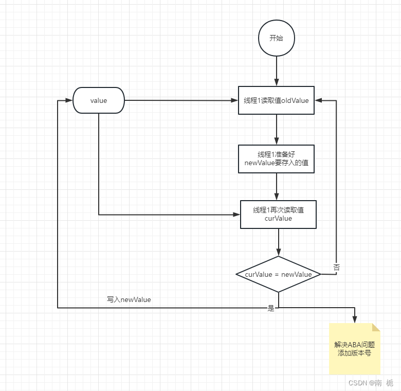
[特殊字符] 手撸 Redis 互斥锁那些坑
📖 手撸 Redis 互斥锁那些坑 最近搞业务遇到高并发下同一个 key 的互斥操作,想实现分布式环境下的互斥锁。于是私下顺手手撸了个基于 Redis 的简单互斥锁,也顺便跟 Redisson 的 RLock 机制对比了下,记录一波,别踩我踩过…...