【深度学习】DDPM,Diffusion,概率扩散去噪生成模型,原理解读
看过来看过去,唯有此up主,非常牛:
Video Explaination(Chinese)
1. DDPM Introduction
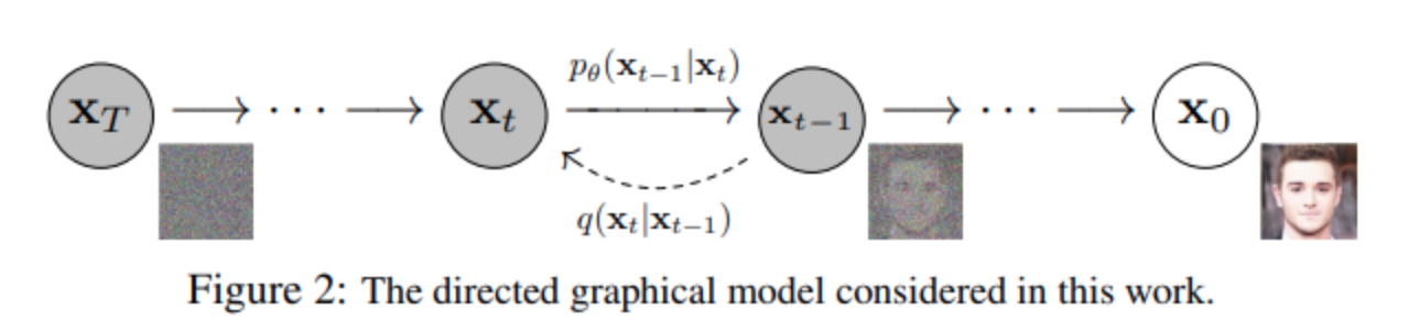
q q q - 一个固定(或预定义)的正向扩散过程,逐渐向图像添加高斯噪声,直到最终得到纯噪声。
p θ p_θ pθ - 一个学习到的反向去噪扩散过程,其中神经网络被训练以逐渐去噪图像,从纯噪声开始,直到最终得到实际图像。
正向和反向过程都由 t t t索引,发生在有限时间步数 T T T内(DDPM的作者使用 T T T=1000)。您从 t = 0 t=0 t=0开始,从数据分布中采样一个真实图像 x 0 x_0 x0,正向过程在每个时间步 t t t中从高斯分布中采样一些噪声,然后将其添加到前一个时间步的图像上。在足够大的 T T T和每个时间步添加噪声的良好安排下,通过逐渐的过程,最终在 t = T t=T t=T处得到所谓的各向同性高斯分布。
2. Forward Process q q q
这个过程是一个马尔可夫链, x t x_t xt 只依赖于 x t − 1 x_{t-1} xt−1。 q ( x t ∣ x t − 1 ) q(x_{t} | x_{t-1}) q(xt∣xt−1) 在每个时间步 t t t 按照已知的方差计划 β t β_{t} βt 添加高斯噪声。
x 0 → q ( x 1 ∣ x 0 ) x 1 → q ( x 2 ∣ x 1 ) x 2 → ⋯ → x T − 1 → q ( x t ∣ x t − 1 ) x T x_0 \overset{q(x_1 | x_0)}{\rightarrow} x_1 \overset{q(x_2 | x_1)}{\rightarrow} x_2 \rightarrow \dots \rightarrow x_{T-1} \overset{q(x_{t} | x_{t-1})}{\rightarrow} x_T x0→q(x1∣x0)x1→q(x2∣x1)x2→⋯→xT−1→q(xt∣xt−1)xT
x t = 1 − β t × x t − 1 + β t × ϵ t x_t = \sqrt{1-β_t}\times x_{t-1} + \sqrt{β_t}\times ϵ_{t} xt=1−βt×xt−1+βt×ϵt
- β t β_t βt is not constant at each time step t t t. In fact one defines a so-called “variance schedule”, which can be linear, quadratic, cosine, etc.
0 < β 1 < β 2 < β 3 < ⋯ < β T < 1 0 < β_1 < β_2 < β_3 < \dots < β_T < 1 0<β1<β2<β3<⋯<βT<1
- ϵ t ϵ_{t} ϵt Gaussian noise, sampled from standard normal distribution.
x t = 1 − β t × x t − 1 + β t × ϵ t x_t = \sqrt{1-β_t}\times x_{t-1} + \sqrt{β_t} \times ϵ_{t} xt=1−βt×xt−1+βt×ϵt
Define a t = 1 − β t a_t = 1 - β_t at=1−βt
x t = a t × x t − 1 + 1 − a t × ϵ t x_t = \sqrt{a_{t}}\times x_{t-1} + \sqrt{1-a_t} \times ϵ_{t} xt=at×xt−1+1−at×ϵt
2.1 Relationship between x t x_t xt and x t − 2 x_{t-2} xt−2
x t − 1 = a t − 1 × x t − 2 + 1 − a t − 1 × ϵ t − 1 x_{t-1} = \sqrt{a_{t-1}}\times x_{t-2} + \sqrt{1-a_{t-1}} \times ϵ_{t-1} xt−1=at−1×xt−2+1−at−1×ϵt−1
⇓ \Downarrow ⇓
x t = a t ( a t − 1 × x t − 2 + 1 − a t − 1 ϵ t − 1 ) + 1 − a t × ϵ t x_t = \sqrt{a_{t}} (\sqrt{a_{t-1}}\times x_{t-2} + \sqrt{1-a_{t-1}} ϵ_{t-1}) + \sqrt{1-a_t} \times ϵ_t xt=at(at−1×xt−2+1−at−1ϵt−1)+1−at×ϵt
⇓ \Downarrow ⇓
x t = a t a t − 1 × x t − 2 + a t ( 1 − a t − 1 ) ϵ t − 1 + 1 − a t × ϵ t x_t = \sqrt{a_{t}a_{t-1}}\times x_{t-2} + \sqrt{a_{t}(1-a_{t-1})} ϵ_{t-1} + \sqrt{1-a_t} \times ϵ_t xt=atat−1×xt−2+at(1−at−1)ϵt−1+1−at×ϵt
Because $N(\mu_{1},\sigma_{1}^{2}) + N(\mu_{2},\sigma_{2}^{2}) = N(\mu_{1}+\mu_{2},\sigma_{1}^{2} + \sigma_{2}^{2})$Proof
x t = a t a t − 1 × x t − 2 + a t ( 1 − a t − 1 ) + 1 − a t × ϵ x_t = \sqrt{a_{t}a_{t-1}}\times x_{t-2} + \sqrt{a_{t}(1-a_{t-1}) + 1-a_t} \times ϵ xt=atat−1×xt−2+at(1−at−1)+1−at×ϵ
⇓ \Downarrow ⇓
x t = a t a t − 1 × x t − 2 + 1 − a t a t − 1 × ϵ x_t = \sqrt{a_{t}a_{t-1}}\times x_{t-2} + \sqrt{1-a_{t}a_{t-1}} \times ϵ xt=atat−1×xt−2+1−atat−1×ϵ
2.2 Relationship between x t x_t xt and x t − 3 x_{t-3} xt−3
x t − 2 = a t − 2 × x t − 3 + 1 − a t − 2 × ϵ t − 2 x_{t-2} = \sqrt{a_{t-2}}\times x_{t-3} + \sqrt{1-a_{t-2}} \times ϵ_{t-2} xt−2=at−2×xt−3+1−at−2×ϵt−2
⇓ \Downarrow ⇓
x t = a t a t − 1 ( a t − 2 × x t − 3 + 1 − a t − 2 ϵ t − 2 ) + 1 − a t a t − 1 × ϵ x_t = \sqrt{a_{t}a_{t-1}}(\sqrt{a_{t-2}}\times x_{t-3} + \sqrt{1-a_{t-2}} ϵ_{t-2}) + \sqrt{1-a_{t}a_{t-1}}\times ϵ xt=atat−1(at−2×xt−3+1−at−2ϵt−2)+1−atat−1×ϵ
⇓ \Downarrow ⇓
x t = a t a t − 1 a t − 2 × x t − 3 + a t a t − 1 ( 1 − a t − 2 ) ϵ t − 2 + 1 − a t a t − 1 × ϵ x_t = \sqrt{a_{t}a_{t-1}a_{t-2}}\times x_{t-3} + \sqrt{a_{t}a_{t-1}(1-a_{t-2})} ϵ_{t-2} + \sqrt{1-a_{t}a_{t-1}}\times ϵ xt=atat−1at−2×xt−3+atat−1(1−at−2)ϵt−2+1−atat−1×ϵ
⇓ \Downarrow ⇓
x t = a t a t − 1 a t − 2 × x t − 3 + a t a t − 1 − a t a t − 1 a t − 2 ϵ t − 2 + 1 − a t a t − 1 × ϵ x_t = \sqrt{a_{t}a_{t-1}a_{t-2}}\times x_{t-3} + \sqrt{a_{t}a_{t-1}-a_{t}a_{t-1}a_{t-2}} ϵ_{t-2} + \sqrt{1-a_{t}a_{t-1}}\times ϵ xt=atat−1at−2×xt−3+atat−1−atat−1at−2ϵt−2+1−atat−1×ϵ
⇓ \Downarrow ⇓
x t = a t a t − 1 a t − 2 × x t − 3 + ( a t a t − 1 − a t a t − 1 a t − 2 ) + 1 − a t a t − 1 × ϵ x_t = \sqrt{a_{t}a_{t-1}a_{t-2}}\times x_{t-3} + \sqrt{(a_{t}a_{t-1}-a_{t}a_{t-1}a_{t-2}) + 1-a_{t}a_{t-1}} \times ϵ xt=atat−1at−2×xt−3+(atat−1−atat−1at−2)+1−atat−1×ϵ
⇓ \Downarrow ⇓
x t = a t a t − 1 a t − 2 × x t − 3 + 1 − a t a t − 1 a t − 2 × ϵ x_t = \sqrt{a_{t}a_{t-1}a_{t-2}}\times x_{t-3} + \sqrt{1-a_{t}a_{t-1}a_{t-2}} \times ϵ xt=atat−1at−2×xt−3+1−atat−1at−2×ϵ
2.3 Relationship between x t x_t xt and x 0 x_0 x0
- x t = a t a t − 1 × x t − 2 + 1 − a t a t − 1 × ϵ x_t = \sqrt{a_{t}a_{t-1}}\times x_{t-2} + \sqrt{1-a_{t}a_{t-1}}\times ϵ xt=atat−1×xt−2+1−atat−1×ϵ
- x t = a t a t − 1 a t − 2 × x t − 3 + 1 − a t a t − 1 a t − 2 × ϵ x_t = \sqrt{a_{t}a_{t-1}a_{t-2}}\times x_{t-3} + \sqrt{1-a_{t}a_{t-1}a_{t-2}}\times ϵ xt=atat−1at−2×xt−3+1−atat−1at−2×ϵ
- x t = a t a t − 1 a t − 2 a t − 3 . . . a t − ( k − 2 ) a t − ( k − 1 ) × x t − k + 1 − a t a t − 1 a t − 2 a t − 3 . . . a t − ( k − 2 ) a t − ( k − 1 ) × ϵ x_t = \sqrt{a_{t}a_{t-1}a_{t-2}a_{t-3}...a_{t-(k-2)}a_{t-(k-1)}}\times x_{t-k} + \sqrt{1-a_{t}a_{t-1}a_{t-2}a_{t-3}...a_{t-(k-2)}a_{t-(k-1)}}\times ϵ xt=atat−1at−2at−3...at−(k−2)at−(k−1)×xt−k+1−atat−1at−2at−3...at−(k−2)at−(k−1)×ϵ
- x t = a t a t − 1 a t − 2 a t − 3 . . . a 2 a 1 × x 0 + 1 − a t a t − 1 a t − 2 a t − 3 . . . a 2 a 1 × ϵ x_t = \sqrt{a_{t}a_{t-1}a_{t-2}a_{t-3}...a_{2}a_{1}}\times x_{0} + \sqrt{1-a_{t}a_{t-1}a_{t-2}a_{t-3}...a_{2}a_{1}}\times ϵ xt=atat−1at−2at−3...a2a1×x0+1−atat−1at−2at−3...a2a1×ϵ
a ˉ t : = a t a t − 1 a t − 2 a t − 3 . . . a 2 a 1 \bar{a}_{t} := a_{t}a_{t-1}a_{t-2}a_{t-3}...a_{2}a_{1} aˉt:=atat−1at−2at−3...a2a1
x t = a ˉ t × x 0 + 1 − a ˉ t × ϵ , ϵ ∼ N ( 0 , I ) x_{t} = \sqrt{\bar{a}_t}\times x_0+ \sqrt{1-\bar{a}_t}\times ϵ , ϵ \sim N(0,I) xt=aˉt×x0+1−aˉt×ϵ,ϵ∼N(0,I)
⇓ \Downarrow ⇓
q ( x t ∣ x 0 ) = 1 2 π 1 − a ˉ t e ( − 1 2 ( x t − a ˉ t x 0 ) 2 1 − a ˉ t ) q(x_{t}|x_{0}) = \frac{1}{\sqrt{2\pi } \sqrt{1-\bar{a}_{t}}} e^{\left ( -\frac{1}{2}\frac{(x_{t}-\sqrt{\bar{a}_{t}}x_0)^2}{1-\bar{a}_{t}} \right ) } q(xt∣x0)=2π1−aˉt1e(−211−aˉt(xt−aˉtx0)2)
3.Reverse Process p p p
Because P ( A ∣ B ) = P ( B ∣ A ) P ( A ) P ( B ) P(A|B) = \frac{ P(B|A)P(A) }{ P(B) } P(A∣B)=P(B)P(B∣A)P(A)
p ( x t − 1 ∣ x t , x 0 ) = q ( x t ∣ x t − 1 , x 0 ) × q ( x t − 1 ∣ x 0 ) q ( x t ∣ x 0 ) p(x_{t-1}|x_{t},x_{0}) = \frac{ q(x_{t}|x_{t-1},x_{0})\times q(x_{t-1}|x_0)}{q(x_{t}|x_0)} p(xt−1∣xt,x0)=q(xt∣x0)q(xt∣xt−1,x0)×q(xt−1∣x0)
| $$x_{t} = \sqrt{a_t}x_{t-1}+\sqrt{1-a_t}\times ϵ$$ | ~ | $N(\sqrt{a_t}x_{t-1}, 1-a_{t})$ |
| $$x_{t-1} = \sqrt{\bar{a}_{t-1}}x_0+ \sqrt{1-\bar{a}_{t-1}}\times ϵ$$ | ~ | $N( \sqrt{\bar{a}_{t-1}}x_0, 1-\bar{a}_{t-1})$ |
| $$x_{t} = \sqrt{\bar{a}_{t}}x_0+ \sqrt{1-\bar{a}_{t}}\times ϵ$$ | ~ | $N( \sqrt{\bar{a}_{t}}x_0, 1-\bar{a}_{t})$ |
q ( x t ∣ x t − 1 , x 0 ) = 1 2 π 1 − a t e ( − 1 2 ( x t − a t x t − 1 ) 2 1 − a t ) q(x_{t}|x_{t-1},x_{0}) = \frac{1}{\sqrt{2\pi } \sqrt{1-a_{t}}} e^{\left ( -\frac{1}{2}\frac{(x_{t}-\sqrt{a_t}x_{t-1})^2}{1-a_{t}} \right ) } q(xt∣xt−1,x0)=2π1−at1e(−211−at(xt−atxt−1)2)
q ( x t − 1 ∣ x 0 ) = 1 2 π 1 − a ˉ t − 1 e ( − 1 2 ( x t − 1 − a ˉ t − 1 x 0 ) 2 1 − a ˉ t − 1 ) q(x_{t-1}|x_{0}) = \frac{1}{\sqrt{2\pi } \sqrt{1-\bar{a}_{t-1}}} e^{\left ( -\frac{1}{2}\frac{(x_{t-1}-\sqrt{\bar{a}_{t-1}}x_0)^2}{1-\bar{a}_{t-1}} \right ) } q(xt−1∣x0)=2π1−aˉt−11e(−211−aˉt−1(xt−1−aˉt−1x0)2)
q ( x t ∣ x 0 ) = 1 2 π 1 − a ˉ t e ( − 1 2 ( x t − a ˉ t x 0 ) 2 1 − a ˉ t ) q(x_{t}|x_{0}) = \frac{1}{\sqrt{2\pi } \sqrt{1-\bar{a}_{t}}} e^{\left ( -\frac{1}{2}\frac{(x_{t}-\sqrt{\bar{a}_{t}}x_0)^2}{1-\bar{a}_{t}} \right ) } q(xt∣x0)=2π1−aˉt1e(−211−aˉt(xt−aˉtx0)2)
q ( x t ∣ x t − 1 , x 0 ) × q ( x t − 1 ∣ x 0 ) q ( x t ∣ x 0 ) = [ 1 2 π 1 − a t e ( − 1 2 ( x t − a t x t − 1 ) 2 1 − a t ) ] ∗ [ 1 2 π 1 − a ˉ t − 1 e ( − 1 2 ( x t − 1 − a ˉ t − 1 x 0 ) 2 1 − a ˉ t − 1 ) ] ÷ [ 1 2 π 1 − a ˉ t e ( − 1 2 ( x t − a ˉ t x 0 ) 2 1 − a ˉ t ) ] \frac{ q(x_{t}|x_{t-1},x_{0})\times q(x_{t-1}|x_0)}{q(x_{t}|x_0)} = \left [ \frac{1}{\sqrt{2\pi} \sqrt{1-a_{t}}} e^{\left ( -\frac{1}{2}\frac{(x_{t}-\sqrt{a_t}x_{t-1})^2}{1-a_{t}} \right ) } \right ] * \left [ \frac{1}{\sqrt{2\pi} \sqrt{1-\bar{a}_{t-1}}} e^{\left ( -\frac{1}{2}\frac{(x_{t-1}-\sqrt{\bar{a}_{t-1}}x_0)^2}{1-\bar{a}_{t-1}} \right ) } \right ] \div \left [ \frac{1}{\sqrt{2\pi} \sqrt{1-\bar{a}_{t}}} e^{\left ( -\frac{1}{2}\frac{(x_{t}-\sqrt{\bar{a}_{t}}x_0)^2}{1-\bar{a}_{t}} \right ) } \right ] q(xt∣x0)q(xt∣xt−1,x0)×q(xt−1∣x0)=[2π1−at1e(−211−at(xt−atxt−1)2)]∗[2π1−aˉt−11e(−211−aˉt−1(xt−1−aˉt−1x0)2)]÷[2π1−aˉt1e(−211−aˉt(xt−aˉtx0)2)]
⇓ \Downarrow ⇓
2 π 1 − a ˉ t 2 π 1 − a t 2 π 1 − a ˉ t − 1 e [ − 1 2 ( ( x t − a t x t − 1 ) 2 1 − a t + ( x t − 1 − a ˉ t − 1 x 0 ) 2 1 − a ˉ t − 1 − ( x t − a ˉ t x 0 ) 2 1 − a ˉ t ) ] \frac{\sqrt{2\pi} \sqrt{1-\bar{a}_{t}}}{\sqrt{2\pi} \sqrt{1-a_{t}} \sqrt{2\pi} \sqrt{1-\bar{a}_{t-1}} } e^{\left [ -\frac{1}{2} \left ( \frac{(x_{t}-\sqrt{a_t}x_{t-1})^2}{1-a_{t}} + \frac{(x_{t-1}-\sqrt{\bar{a}_{t-1}}x_0)^2}{1-\bar{a}_{t-1}} - \frac{(x_{t}-\sqrt{\bar{a}_{t}}x_0)^2}{1-\bar{a}_{t}} \right ) \right ] } 2π1−at2π1−aˉt−12π1−aˉte[−21(1−at(xt−atxt−1)2+1−aˉt−1(xt−1−aˉt−1x0)2−1−aˉt(xt−aˉtx0)2)]
⇓ \Downarrow ⇓
1 2 π ( 1 − a t 1 − a ˉ t − 1 1 − a ˉ t ) e x p [ − 1 2 ( ( x t − a t x t − 1 ) 2 1 − a t + ( x t − 1 − a ˉ t − 1 x 0 ) 2 1 − a ˉ t − 1 − ( x t − a ˉ t x 0 ) 2 1 − a ˉ t ) ] \frac{1}{\sqrt{2\pi} \left ( \frac{ \sqrt{1-a_t} \sqrt{1-\bar{a}_{t-1}} } {\sqrt{1-\bar{a}_{t}}} \right ) } exp{\left [ -\frac{1}{2} \left ( \frac{(x_{t}-\sqrt{a_t}x_{t-1})^2}{1-a_t} + \frac{(x_{t-1}-\sqrt{\bar{a}_{t-1}}x_0)^2}{1-\bar{a}_{t-1}} - \frac{(x_{t}-\sqrt{\bar{a}_{t}}x_0)^2}{1-\bar{a}_{t}} \right ) \right ] } 2π(1−aˉt1−at1−aˉt−1)1exp[−21(1−at(xt−atxt−1)2+1−aˉt−1(xt−1−aˉt−1x0)2−1−aˉt(xt−aˉtx0)2)]
⇓ \Downarrow ⇓
1 2 π ( 1 − a t 1 − a ˉ t − 1 1 − a ˉ t ) e x p [ − 1 2 ( x t 2 − 2 a t x t x t − 1 + a t x t − 1 2 1 − a t + x t − 1 2 − 2 a ˉ t − 1 x 0 x t − 1 + a ˉ t − 1 x 0 2 1 − a ˉ t − 1 − ( x t − a ˉ t x 0 ) 2 1 − a ˉ t ) ] \frac{1}{\sqrt{2\pi} \left ( \frac{ \sqrt{1-a_t} \sqrt{1-\bar{a}_{t-1}} } {\sqrt{1-\bar{a}_{t}}} \right ) } exp \left[ -\frac{1}{2} \left ( \frac{ x_{t}^2-2\sqrt{a_t}x_{t}x_{t-1}+{a_t}x_{t-1}^2 }{1-a_t} + \frac{ x_{t-1}^2-2\sqrt{\bar{a}_{t-1}}x_0x_{t-1}+\bar{a}_{t-1}x_0^2 }{1-\bar{a}_{t-1}} - \frac{(x_{t}-\sqrt{\bar{a}_{t}}x_0)^2}{1-\bar{a}_{t}} \right) \right] 2π(1−aˉt1−at1−aˉt−1)1exp[−21(1−atxt2−2atxtxt−1+atxt−12+1−aˉt−1xt−12−2aˉt−1x0xt−1+aˉt−1x02−1−aˉt(xt−aˉtx0)2)]
⇓ \Downarrow ⇓
1 2 π ( 1 − a t 1 − a ˉ t − 1 1 − a ˉ t ) e x p [ − 1 2 ( x t − 1 − ( a t ( 1 − a ˉ t − 1 ) 1 − a ˉ t x t + a ˉ t − 1 ( 1 − a t ) 1 − a ˉ t x 0 ) ) 2 ( 1 − a t 1 − a ˉ t − 1 1 − a ˉ t ) 2 ] \frac{1}{\sqrt{2\pi} \left ( {\color{Red} \frac{ \sqrt{1-a_t} \sqrt{1-\bar{a}_{t-1}} } {\sqrt{1-\bar{a}_{t}}}} \right ) } exp \left[ -\frac{1}{2} \frac{ \left( x_{t-1} - \left( {\color{Purple} \frac{\sqrt{a_t}(1-\bar{a}_{t-1})}{1-\bar{a}_t}x_t + \frac{\sqrt{\bar{a}_{t-1}}(1-a_t)}{1-\bar{a}_t}x_0} \right) \right) ^2 } { \left( {\color{Red} \frac{ \sqrt{1-a_t} \sqrt{1-\bar{a}_{t-1}} } {\sqrt{1-\bar{a}_{t}}}} \right)^2 } \right] 2π(1−aˉt1−at1−aˉt−1)1exp −21(1−aˉt1−at1−aˉt−1)2(xt−1−(1−aˉtat(1−aˉt−1)xt+1−aˉtaˉt−1(1−at)x0))2
⇓ \Downarrow ⇓
p ( x t − 1 ∣ x t ) ∼ N ( a t ( 1 − a ˉ t − 1 ) 1 − a ˉ t x t + a ˉ t − 1 ( 1 − a t ) 1 − a ˉ t x 0 , ( 1 − a t 1 − a ˉ t − 1 1 − a ˉ t ) 2 ) p(x_{t-1}|x_{t}) \sim N\left( {\color{Purple} \frac{\sqrt{a_t}(1-\bar{a}_{t-1})}{1-\bar{a}_t}x_t + \frac{\sqrt{\bar{a}_{t-1}}(1-a_t)}{1-\bar{a}_t}x_0} , \left( {\color{Red} \frac{ \sqrt{1-a_t} \sqrt{1-\bar{a}_{t-1}} } {\sqrt{1-\bar{a}_{t}}}} \right)^2 \right) p(xt−1∣xt)∼N(1−aˉtat(1−aˉt−1)xt+1−aˉtaˉt−1(1−at)x0,(1−aˉt1−at1−aˉt−1)2)
Because x t = a ˉ t × x 0 + 1 − a ˉ t × ϵ x_{t} = \sqrt{\bar{a}_t}\times x_0+ \sqrt{1-\bar{a}_t}\times ϵ xt=aˉt×x0+1−aˉt×ϵ, x 0 = x t − 1 − a ˉ t × ϵ a ˉ t x_0 = \frac{x_t - \sqrt{1-\bar{a}_t}\times ϵ}{\sqrt{\bar{a}_t}} x0=aˉtxt−1−aˉt×ϵ. Substitute x 0 x_0 x0 with this formula.
p ( x t − 1 ∣ x t ) ∼ N ( a t ( 1 − a ˉ t − 1 ) 1 − a ˉ t x t + a ˉ t − 1 ( 1 − a t ) 1 − a ˉ t × x t − 1 − a ˉ t × ϵ a ˉ t , β t ( 1 − a ˉ t − 1 ) 1 − a ˉ t ) p(x_{t-1}|x_{t}) \sim N\left( {\color{Purple} \frac{\sqrt{a_t}(1-\bar{a}_{t-1})}{1-\bar{a}_t}x_t + \frac{\sqrt{\bar{a}_{t-1}}(1-a_t)}{1-\bar{a}_t}\times \frac{x_t - \sqrt{1-\bar{a}_t}\times ϵ}{\sqrt{\bar{a}_t}} } , {\color{Red} \frac{ \beta_{t} (1-\bar{a}_{t-1}) } { 1-\bar{a}_{t}}} \right) p(xt−1∣xt)∼N(1−aˉtat(1−aˉt−1)xt+1−aˉtaˉt−1(1−at)×aˉtxt−1−aˉt×ϵ,1−aˉtβt(1−aˉt−1))
相关文章:
【深度学习】DDPM,Diffusion,概率扩散去噪生成模型,原理解读
看过来看过去,唯有此up主,非常牛: Video Explaination(Chinese) 1. DDPM Introduction q q q - 一个固定(或预定义)的正向扩散过程,逐渐向图像添加高斯噪声,直到最终得到纯噪声。 p θ p_θ p…...
HT8699:内置 BOOST 升Y双声道音频功率放大器
HT8699是一款内置BOOST升Y模块的立体声音频功率放大器。HT8699具有AB类和D类切换功能,在受到D类功放EMI干扰困扰时,可切换至AB类音频功放模式。 在D类模式下,内置的BOOST升Y模块可通过外置电阻调节升Y值,即使是锂电池供电…...

利达卓越:关注环保事业,持续赋能科技
随着全球环境问题的日益突出,绿色金融作为一种新兴的金融模式逐渐受到各国的重视。绿色金融是指在金融活动中,通过资金、信贷和风险管理等手段,支持环境友好和可持续发展的项目和产业。绿色金融的出现是为了应对气候变化、资源短缺、污染问题等现实挑战,促进经济的绿色转型和可…...

Spring MVC中通过配置文件配置定时任务
Spring MVC中配置定时任务(配置文件方式) 1.步骤 1.步骤 1-1 在springmvc.xml(配置文件)的beans中添加 xmlns:task"http://www.springframework.org/schema/task" http://www.springframework.org/schema/task http…...
AI项目十六:YOLOP 训练+测试+模型评估
若该文为原创文章,转载请注明原文出处。 通过正点原子的ATK-3568了解到了YOLOP,这里记录下训练及测试及在onnxruntime部署的过程。 步骤:训练->测试->转成onnx->onnxruntime部署测试 一、前言 YOLOP是华中科技大学研究团队在2021年…...
Flink报错could not be loaded due to a linkage failure
文章目录 1、报错2、原因3、解决 1、报错 在Flink上提交作业,点Submit没反应,F12看到接口报错信息为: 大概意思是,由于链接失败,无法加载程序的入口点类xx。没啥鸟用的信息,去日志目录继续分析:…...

网络工程师--网络安全与应用案例分析
前言 需要网络安全学习资料的点击链接:【282G】网络安全&黑客技术零基础到进阶全套学习大礼包,免费分享! 案例一: 某单位现有网络拓扑结构如下图所示,实现用户上网功能,该网络使用的网络交换机均为三…...
了解油封对汽车安全的影响?
油封也称为轴封或径向轴封,是车辆发动机、变速箱和其他各种机械系统中的重要部件。它们的主要功能是阻止重要发动机部件的液体(例如油或冷却剂)泄漏,同时防止污染物进入。这些看似简单的任务,但对汽车的安全性和可靠性有着深远的影响。 油封…...

创邻科技Galaxybase—激活数据要素的核心引擎
10月11日下午,创邻科技创始人张晨博士受杭州电子科技大学邀请,前往杭电校园开展交流分享。交流会中,张晨博士为现场的师生带来一场题为《图数据库——激活数据要素的新基建》的精彩分享,探讨数字经济时代底层技术的创新价值与图技…...
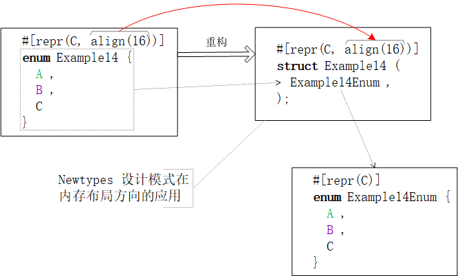
【Rust笔记】浅聊 Rust 程序内存布局
浅聊Rust程序内存布局 内存布局看似是底层和距离应用程序开发比较遥远的概念集合,但其对前端应用的功能实现颇具现实意义。从WASM业务模块至Nodejs N-API插件,无处不涉及到FFI跨语言互操作。甚至,做个文本数据的字符集转换也得FFI调用操作系统…...
玻璃生产过程中的窑内压力高精度恒定控制解决方案
摘要:在玻璃生产中对玻璃窑炉中窑压的要求极高,通常需要控制微正压4.7Pa(表压),偏差控制在0.3Pa,而窑炉压力还会受到众多因素的影响,所以实现高稳定性的熔窑压力控制具有很大难度,为…...

创意营销:初期推广的多种策略!
文章目录 🍊 预热🎉 制定预热计划和目标🎉 利用社交媒体传播🎉 创造独特的体验🎉 利用口碑营销🎉 定期发布更新信息🎉 案例说明 🍊 小范围推广🎉 明确目标用户群体&#…...
【小黑嵌入式系统第一课】嵌入式系统的概述(一)
文章目录 一、嵌入式系统基本概念计算机发展的三大阶段CPU——计算机的核心什么是嵌入式系统嵌入式系统的分类 二、嵌入式系统的特点三、嵌入式系统发展无操作系统阶段简单操作系统阶段实时操作系统阶段面向Internet阶段 四、嵌入式系统的应用工业控制 工业设备通信设备信息家电…...
RK平台使用MP4视频做开机动画以及卡顿问题
rk平台android11以后系统都可以使用MP4格式的视频做开机动画,系统源码里面默认使用的是ts格式的视频,其实使用mp4的视频也是可以的。具体修改如下: diff --git a/frameworks/base/cmds/bootanimation/BootAnimation.cpp b/frameworks/base/cmds/bootanimation/BootAnimat…...
通讯网关软件023——利用CommGate X2HTTP实现HTTP访问Modbus TCP
本文介绍利用CommGate X2HTTP实现HTTP访问Modbus TCP。CommGate X2HTTP是宁波科安网信开发的网关软件,软件可以登录到网信智汇(http://wangxinzhihui.com)下载。 【案例】如下图所示,SCADA系统上位机、PLC、设备具备Modbus RTU通讯接口,现在…...

Python性能测试框架Locust实战教程!
01、认识Locust Locust是一个比较容易上手的分布式用户负载测试工具。它旨在对网站(或其他系统)进行负载测试,并确定系统可以处理多少个并发用户,Locust 在英文中是 蝗虫 的意思:作者的想法是在测试期间,放…...
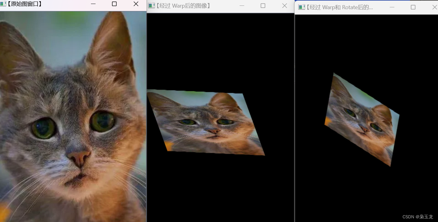
c++视觉处理---仿射变换和二维旋转变换矩阵的函数
仿射变换cv::warpAffine cv::warpAffine 是OpenCV中用于执行仿射变换的函数。仿射变换是一种线性变换,可用于执行平移、旋转、缩放和剪切等操作。下面是 cv::warpAffine 函数的基本用法: cv::warpAffine(src, dst, M, dsize, flags, borderMode, borde…...
uiautomator2遍历子元素.all()
当你获取了页面某个元素之后 elements d(’//*[clickable“true”]’).all() 返回的是一个list,其中是<uiautomator2.xpath.XMLElement>类型的变量。 可以通过以下方式获取它所有子类的信息。 for ele in elements:children ele.elem.getchildren()注意…...
【手写数据库toadb】SQL字符串如何被数据库认识? 词法语法分析基础原理,常用工具
词法语法分析 专栏内容: 手写数据库toadb 本专栏主要介绍如何从零开发,开发的步骤,以及开发过程中的涉及的原理,遇到的问题等,让大家能跟上并且可以一起开发,让每个需要的人成为参与者。 本专栏会定期更新,对应的代码也会定期更新,每个阶段的代码会打上tag,方便阶段…...

手把手教你基于windows系统使用GNVM进行node切换版本
GNVM是什么? GNVM 是一个简单的 Windows 下 Node.js 多版本管理器,类似的 nvm nvmw nodist 。 安装 进入官网,下载你所需要的包,直达链接 下载完成 放到我们的node环境包下,点击运行 请注意区分: 不存在 Node.js 环…...
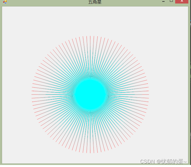
c#画五角星
c#画一个五角星,最重要的就是计算哪些坐标点出来,也是最难的一部分,这要涉及到一些数学方面的知识.对数学坐标知识不是很熟的人,如果想学画图,我建议多去看一下数学书,对我们写程序的人来说是没有什么坏处可言的. 想学习的朋友可以一起学习,我觉得分享学习是一种快乐,所以把自…...
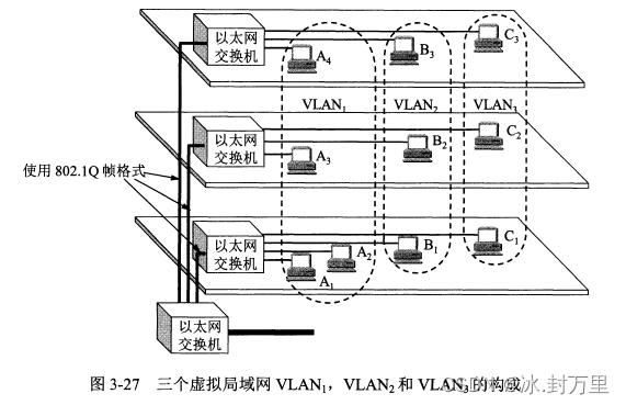
第三章 数据链路层 | 计算机网络(谢希仁 第八版)
文章目录 第三章 数据链路层3.1 使用点对点信道的数据链路层3.1.1 数据链路和帧3.1.2 三个基本问题 3.2 点对点协议PPP3.2.1 PPP协议的特点3.2.2 PPP协议的帧格式3.2.3 PPP协议的工作状态 3.3 使用广播信道的数据链路层3.3.1 局域网的数据链路层3.3.2 CSMA/CD协议3.3.3 使用集线…...
李沐机器学习环境配置相关
李沐机器学习环境配置相关 condapython环境安装指令安装miniconda安装cpu版本torch安装jupyter测试GPU是否可以使用 conda 退出 conda 环境 conda deactivate进入都d2l环境 conda activate d2l启动jupyter notebook: jupyter notebookpython 列出所有安装的包 pip lsit环…...
零基础Linux_16(基础IO_文件)笔试选择题:文件描述符+ionde和动静态库
目录 一. 文件描述符等 1. Linux下两个进程可以同时打开同一个文件,这时如下描述错误的是: 2. 以下关于标准输入输出错误的描述正确的是 3. 以下描述正确的是 4. 以下描述正确的是 [多选] 5. 在bash中,在一条命令后加入”1>&2”…...
基于OpenCV的灰度图的图片相似度计算
from skimage.metrics import structural_similarity as ssim import matplotlib.pyplot as plt import cv2 def picture_recognization(imagname):# 读取两张图片image1 cv2.imread(D:/AutoTest/PythonProject/standard_img/ imagname)image2 cv2.imread(D:/AutoTest/Pytho…...
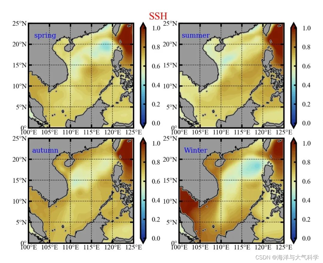
【python海洋专题二十】subplots_adjust布局调整
上期读取soda,并subplot 但是存在一些不完美,本期修饰 本期内容 subplots_adjust布局调整 1:未调整布局的 2:调整布局 往期推荐 【python海洋专题一】查看数据nc文件的属性并输出属性到txt文件 【python海洋专题二】读取水深…...
TensorFlow入门(二十四、初始化学习参数)
参数的初始化关系到网络能否训练出好的结果或者是以多快的速度收敛,对训练结果有着重要的影响。 初始化学习参数需要注意的规则 不可以将网络中的所有参数初始化为0,也不能全部初始化为同一个值。如果参数全部初始化为0或者是同一个值,会使得所有神经元的输出都是相同的,进而造…...

工厂WMS系统货架位管理:优化仓储效率
货架位管理作为WMS系统中的重要环节,对于提高工厂的仓储效率和精确库存管理至关重要。本文将从多个角度全方位介绍工厂的WMS系统货架位管理,探讨其重要性以及如何优化、应用该系统,提升工厂的仓储效率和运营水平。 1. 优化仓库空间利用&…...
[C++随想录] 继承
继承 继承的引言基类和子类的赋值转换继承中的作用域派生类中的默认成员函数继承与友元继承与静态成员多继承的结构棱形继承的结构棱形虚拟继承的结构继承与组合 继承的引言 概念 继承(inheritance)机制是面向对象程序设计使代码可以 复用的最重要的手段,它允许程序…...
ARM-day9
按键控制小灯、蜂鸣器、风扇,按一次启动,第二次关闭 key_it.c #include "key_it.h"//按键3的配置 void key3_it_config() {//RCC使能GPIOF时钟RCC->MP_AHB4ENSETR | (0x1<<5);GPIOF->MODER & (~(0x3<<16));EXTI->E…...