企业级实战项目:基于 pycaret 自动化预测公司是否破产
本文系数据挖掘实战系列文章,我跟大家分享一个数据挖掘实战,与以往的数据实战不同的是,用自动机器学习方法完成模型构建与调优部分工作,深入理解由此带来的便利与效果。
1. Introduction
本文是一篇数据挖掘实战案例,详细探索了从台湾经济杂志收集的1999年到2009年的数据,看看在数据探索过程中,可以洞察出哪些有用的信息,判断哪一个模型能够最准确地预测公司是否破产。
公司破产的定义是根据台湾证券交易所的商业规则而定的。
该建模将尝试使用自动机器学习库pycaret来构建机器学习模型,pycaret是一个用python编写的开源低代码机器学习库,它将机器学习工作流程自动化。如果你想探索这个库并更好地理解它的功能。推荐查看
设置环境并读取数据
import pandas as pd
import numpy as np
import math
import matplotlib.pyplot as plt
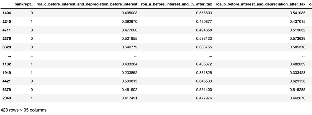
import seaborn as sns bankruptcy_df = pd.read_csv("Bankruptcy.csv") bankruptcy_df.head()
技术交流&源码获取
技术要学会交流、分享,不建议闭门造车。一个人可以走的很快、一堆人可以走的更远。
好的文章离不开粉丝的分享、推荐,资料干货、资料分享、数据、技术交流提升,均可加交流群获取,群友已超过2000人,添加时最好的备注方式为:来源+兴趣方向,方便找到志同道合的朋友。
本文数据&源码,技术交流、按照如下方式获取:
方式①、添加微信号:dkl88194,备注:资料
方式②、微信搜索公众号:Python学习与数据挖掘,后台回复:资料
资料1

资料2
我们打造了《100个超强算法模型》,特点:从0到1轻松学习,原理、代码、案例应有尽有,所有的算法模型都是按照这样的节奏进行表述,所以是一套完完整整的案例库。
很多初学者是有这么一个痛点,就是案例,案例的完整性直接影响同学的兴致。因此,我整理了 100个最常见的算法模型,在你的学习路上助推一把!

2. 理解数据
bankruptcy_df.info()
<class 'pandas.core.frame.DataFrame'>
RangeIndex: 6819 entries, 0 to 6818
Data columns (total 96 columns):  #   Column                                                    Non-Null Count  Dtype    ---  ------                                                    --------------  -----  0   Bankrupt?                                                 6819 non-null   int64    1    ROA(C) before interest and depreciation before interest  6819 non-null   float64  2    ROA(A) before interest and % after tax                   6819 non-null   float64  3    ROA(B) before interest and depreciation after tax        6819 non-null   float64  4    Operating Gross Margin                                   6819 non-null   float64  5    Realized Sales Gross Margin                              6819 non-null   float64  6    Operating Profit Rate                                    6819 non-null   float64  7    Pre-tax net Interest Rate                                6819 non-null   float64  8    After-tax net Interest Rate                              6819 non-null   float64  9    Non-industry income and expenditure/revenue              6819 non-null   float64  10   Continuous interest rate (after tax)                     6819 non-null   float64  11   Operating Expense Rate                                   6819 non-null   float64  12   Research and development expense rate                    6819 non-null   float64  13   Cash flow rate                                           6819 non-null   float64  14   Interest-bearing debt interest rate                      6819 non-null   float64  15   Tax rate (A)                                             6819 non-null   float64  16   Net Value Per Share (B)                                  6819 non-null   float64  17   Net Value Per Share (A)                                  6819 non-null   float64  18   Net Value Per Share (C)                                  6819 non-null   float64  19   Persistent EPS in the Last Four Seasons                  6819 non-null   float64  20   Cash Flow Per Share                                      6819 non-null   float64  21   Revenue Per Share (Yuan ¥)                               6819 non-null   float64  22   Operating Profit Per Share (Yuan ¥)                      6819 non-null   float64  23   Per Share Net profit before tax (Yuan ¥)                 6819 non-null   float64  24   Realized Sales Gross Profit Growth Rate                  6819 non-null   float64  25   Operating Profit Growth Rate                             6819 non-null   float64  26   After-tax Net Profit Growth Rate                         6819 non-null   float64  27   Regular Net Profit Growth Rate                           6819 non-null   float64  28   Continuous Net Profit Growth Rate                        6819 non-null   float64  29   Total Asset Growth Rate                                  6819 non-null   float64  30   Net Value Growth Rate                                    6819 non-null   float64  31   Total Asset Return Growth Rate Ratio                     6819 non-null   float64  32   Cash Reinvestment %                                      6819 non-null   float64  33   Current Ratio                                            6819 non-null   float64  34   Quick Ratio                                              6819 non-null   float64  35   Interest Expense Ratio                                   6819 non-null   float64  36   Total debt/Total net worth                               6819 non-null   float64  37   Debt ratio %                                             6819 non-null   float64  38   Net worth/Assets                                         6819 non-null   float64  39   Long-term fund suitability ratio (A)                     6819 non-null   float64  40   Borrowing dependency                                     6819 non-null   float64  41   Contingent liabilities/Net worth                         6819 non-null   float64  42   Operating profit/Paid-in capital                         6819 non-null   float64  43   Net profit before tax/Paid-in capital                    6819 non-null   float64  44   Inventory and accounts receivable/Net value              6819 non-null   float64  45   Total Asset Turnover                                     6819 non-null   float64  46   Accounts Receivable Turnover                             6819 non-null   float64  47   Average Collection Days                                  6819 non-null   float64  48   Inventory Turnover Rate (times)                          6819 non-null   float64  49   Fixed Assets Turnover Frequency                          6819 non-null   float64  50   Net Worth Turnover Rate (times)                          6819 non-null   float64  51   Revenue per person                                       6819 non-null   float64  52   Operating profit per person                              6819 non-null   float64  53   Allocation rate per person                               6819 non-null   float64  54   Working Capital to Total Assets                          6819 non-null   float64  55   Quick Assets/Total Assets                                6819 non-null   float64  56   Current Assets/Total Assets                              6819 non-null   float64  57   Cash/Total Assets                                        6819 non-null   float64  58   Quick Assets/Current Liability                           6819 non-null   float64  59   Cash/Current Liability                                   6819 non-null   float64  60   Current Liability to Assets                              6819 non-null   float64  61   Operating Funds to Liability                             6819 non-null   float64  62   Inventory/Working Capital                                6819 non-null   float64  63   Inventory/Current Liability                              6819 non-null   float64  64   Current Liabilities/Liability                            6819 non-null   float64  65   Working Capital/Equity                                   6819 non-null   float64  66   Current Liabilities/Equity                               6819 non-null   float64  67   Long-term Liability to Current Assets                    6819 non-null   float64  68   Retained Earnings to Total Assets                        6819 non-null   float64  69   Total income/Total expense                               6819 non-null   float64  70   Total expense/Assets                                     6819 non-null   float64  71   Current Asset Turnover Rate                              6819 non-null   float64  72   Quick Asset Turnover Rate                                6819 non-null   float64  73   Working capitcal Turnover Rate                           6819 non-null   float64  74   Cash Turnover Rate                                       6819 non-null   float64  75   Cash Flow to Sales                                       6819 non-null   float64  76   Fixed Assets to Assets                                   6819 non-null   float64  77   Current Liability to Liability                           6819 non-null   float64  78   Current Liability to Equity                              6819 non-null   float64  79   Equity to Long-term Liability                            6819 non-null   float64  80   Cash Flow to Total Assets                                6819 non-null   float64  81   Cash Flow to Liability                                   6819 non-null   float64  82   CFO to Assets                                            6819 non-null   float64  83   Cash Flow to Equity                                      6819 non-null   float64  84   Current Liability to Current Assets                      6819 non-null   float64  85   Liability-Assets Flag                                    6819 non-null   int64    86   Net Income to Total Assets                               6819 non-null   float64  87   Total assets to GNP price                                6819 non-null   float64  88   No-credit Interval                                       6819 non-null   float64  89   Gross Profit to Sales                                    6819 non-null   float64  90   Net Income to Stockholder's Equity                       6819 non-null   float64  91   Liability to Equity                                      6819 non-null   float64  92   Degree of Financial Leverage (DFL)                       6819 non-null   float64  93   Interest Coverage Ratio (Interest expense to EBIT)       6819 non-null   float64  94   Net Income Flag                                          6819 non-null   int64    95   Equity to Liability                                      6819 non-null   float64
dtypes: float64(93), int64(3)
memory usage: 5.0 MB
bankruptcy_df.shape
(6819, 96)
bankruptcy_df.describe()
3. 数据探索与清洗
3.1 缺失值处理
bankruptcy_df.columns[bankruptcy_df.isna().any()]
Index([], dtype='object')
从结果看,改数据集非常完整,没有缺失值!
.any()指的是有没有(缺失值),而与之对应的.all()指的是是否都是(缺失值)
调整数据列名
def clean_col_names(col_name):  col_name = (  col_name.strip()  .replace("?", "_")  .replace("(", "_")  .replace(")", "_")  .replace(" ", "_")  .replace("/", "_")  .replace("-", "_")  .replace("__", "_")  .replace("'", "")  .lower()  )  return col_name  bank_columns = list(bankruptcy_df.columns)
bank_columns = [clean_col_names(col_name) for col_name in bank_columns]
bankruptcy_df.columns = bank_columns
display(bankruptcy_df.columns)
Index(['bankrupt_', 'roa_c_before_interest_and_depreciation_before_interest', 'roa_a_before_interest_and_%_after_tax', 'roa_b_before_interest_and_depreciation_after_tax', 'operating_gross_margin', 'realized_sales_gross_margin', 'operating_profit_rate', 'pre_tax_net_interest_rate', 'after_tax_net_interest_rate', 'non_industry_income_and_expenditure_revenue', 'continuous_interest_rate_after_tax_', 'operating_expense_rate', 'research_and_development_expense_rate', 'cash_flow_rate', 'interest_bearing_debt_interest_rate', 'tax_rate_a_', 'net_value_per_share_b_', 'net_value_per_share_a_', 'net_value_per_share_c_', 'persistent_eps_in_the_last_four_seasons', 'cash_flow_per_share', 'revenue_per_share_yuan_¥_', 'operating_profit_per_share_yuan_¥_', 'per_share_net_profit_before_tax_yuan_¥_', 'realized_sales_gross_profit_growth_rate', 'operating_profit_growth_rate', 'after_tax_net_profit_growth_rate', 'regular_net_profit_growth_rate', 'continuous_net_profit_growth_rate', 'total_asset_growth_rate', 'net_value_growth_rate', 'total_asset_return_growth_rate_ratio', 'cash_reinvestment_%', 'current_ratio', 'quick_ratio', 'interest_expense_ratio', 'total_debt_total_net_worth', 'debt_ratio_%', 'net_worth_assets', 'long_term_fund_suitability_ratio_a_', 'borrowing_dependency', 'contingent_liabilities_net_worth', 'operating_profit_paid_in_capital', 'net_profit_before_tax_paid_in_capital', 'inventory_and_accounts_receivable_net_value', 'total_asset_turnover', 'accounts_receivable_turnover', 'average_collection_days', 'inventory_turnover_rate_times_', 'fixed_assets_turnover_frequency', 'net_worth_turnover_rate_times_', 'revenue_per_person', 'operating_profit_per_person', 'allocation_rate_per_person', 'working_capital_to_total_assets', 'quick_assets_total_assets', 'current_assets_total_assets', 'cash_total_assets', 'quick_assets_current_liability', 'cash_current_liability', 'current_liability_to_assets', 'operating_funds_to_liability', 'inventory_working_capital', 'inventory_current_liability', 'current_liabilities_liability', 'working_capital_equity', 'current_liabilities_equity', 'long_term_liability_to_current_assets', 'retained_earnings_to_total_assets', 'total_income_total_expense', 'total_expense_assets', 'current_asset_turnover_rate', 'quick_asset_turnover_rate', 'working_capitcal_turnover_rate', 'cash_turnover_rate', 'cash_flow_to_sales', 'fixed_assets_to_assets', 'current_liability_to_liability', 'current_liability_to_equity', 'equity_to_long_term_liability', 'cash_flow_to_total_assets', 'cash_flow_to_liability', 'cfo_to_assets', 'cash_flow_to_equity', 'current_liability_to_current_assets', 'liability_assets_flag', 'net_income_to_total_assets', 'total_assets_to_gnp_price', 'no_credit_interval', 'gross_profit_to_sales', 'net_income_to_stockholders_equity', 'liability_to_equity', 'degree_of_financial_leverage_dfl_', 'interest_coverage_ratio_interest_expense_to_ebit_', 'net_income_flag', 'equity_to_liability'], dtype='object')
统计并绘制目标变量
该步骤的目的是查看目标变量是否平衡,如果不平衡,则需要针对性处理。
class_bar=sns.countplot(data=bankruptcy_df,x="bankrupt_")
ax = plt.gca()
for p in ax.patches:  ax.annotate('{:.1f}'.format(p.get_height()), (p.get_x()+0.3, p.get_height()+500))
class_bar
3.2 特征分布
检查偏态
# Return true/false if skewed
import scipy.stats
skew_df = pd.DataFrame(bankruptcy_df.select_dtypes(np.number).columns, columns = ['Feature'])  skew_df['Skew'] = skew_df['Feature'].apply(lambda feature: scipy.stats.skew(bankruptcy_df[feature]))   skew_df['Absolute Skew'] = skew_df['Skew'].apply(abs)
# 得到与方向无关的倾斜幅度
skew_df['Skewed']= skew_df['Absolute Skew'].apply(lambda x: True if x>= 0.5 else False)
with pd.option_context("display.max_rows", 1000):  display(skew_df)
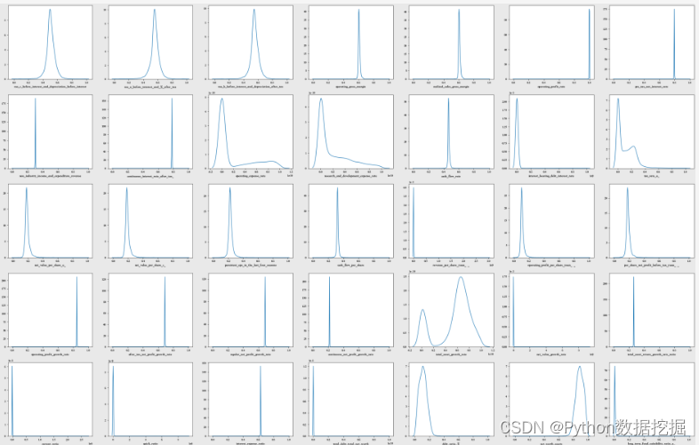
可视化分布
cols = list(bankruptcy_df.columns)
ncols = 8
nrows = math.ceil(len(cols) / ncols)  fig, ax = plt.subplots(nrows, ncols, figsize = (4.5 * ncols, 4 * nrows))
for i in range(len(cols)):  sns.kdeplot(bankruptcy_df[cols[i]], ax = ax[i // ncols, i % ncols])  if i % ncols != 0:  ax[i // ncols, i % ncols].set_ylabel(" ")
plt.tight_layout()
plt.show()
查看有偏态的特征
query_skew=skew_df.query("Skewed == True")["Feature"]
with pd.option_context("display.max_rows", 1000):  display(query_skew)
0                                             bankrupt_
2                 roa_a_before_interest_and_%_after_tax
3      roa_b_before_interest_and_depreciation_after_tax
4                                operating_gross_margin
5                           realized_sales_gross_margin
6                                 operating_profit_rate
7                             pre_tax_net_interest_rate
8                           after_tax_net_interest_rate
9           non_industry_income_and_expenditure_revenue
10                  continuous_interest_rate_after_tax_
11                               operating_expense_rate
12                research_and_development_expense_rate
13                                       cash_flow_rate
14                  interest_bearing_debt_interest_rate
15                                          tax_rate_a_
16                               net_value_per_share_b_
17                               net_value_per_share_a_
18                               net_value_per_share_c_
19              persistent_eps_in_the_last_four_seasons
20                                  cash_flow_per_share
21                            revenue_per_share_yuan_¥_
22                   operating_profit_per_share_yuan_¥_
23              per_share_net_profit_before_tax_yuan_¥_
24              realized_sales_gross_profit_growth_rate
25                         operating_profit_growth_rate
26                     after_tax_net_profit_growth_rate
27                       regular_net_profit_growth_rate
28                    continuous_net_profit_growth_rate
29                              total_asset_growth_rate
30                                net_value_growth_rate
31                 total_asset_return_growth_rate_ratio
32                                  cash_reinvestment_%
33                                        current_ratio
34                                          quick_ratio
35                               interest_expense_ratio
36                           total_debt_total_net_worth
37                                         debt_ratio_%
38                                     net_worth_assets
39                  long_term_fund_suitability_ratio_a_
40                                 borrowing_dependency
41                     contingent_liabilities_net_worth
42                     operating_profit_paid_in_capital
43                net_profit_before_tax_paid_in_capital
44          inventory_and_accounts_receivable_net_value
45                                 total_asset_turnover
46                         accounts_receivable_turnover
47                              average_collection_days
48                       inventory_turnover_rate_times_
49                      fixed_assets_turnover_frequency
50                       net_worth_turnover_rate_times_
51                                   revenue_per_person
52                          operating_profit_per_person
53                           allocation_rate_per_person
57                                    cash_total_assets
58                       quick_assets_current_liability
59                               cash_current_liability
60                          current_liability_to_assets
61                         operating_funds_to_liability
62                            inventory_working_capital
63                          inventory_current_liability
64                        current_liabilities_liability
65                               working_capital_equity
66                           current_liabilities_equity
67                long_term_liability_to_current_assets
68                    retained_earnings_to_total_assets
69                           total_income_total_expense
70                                 total_expense_assets
71                          current_asset_turnover_rate
72                            quick_asset_turnover_rate
73                       working_capitcal_turnover_rate
74                                   cash_turnover_rate
75                                   cash_flow_to_sales
76                               fixed_assets_to_assets
77                       current_liability_to_liability
78                          current_liability_to_equity
79                        equity_to_long_term_liability
81                               cash_flow_to_liability
83                                  cash_flow_to_equity
84                  current_liability_to_current_assets
85                                liability_assets_flag
86                           net_income_to_total_assets
87                            total_assets_to_gnp_price
88                                   no_credit_interval
89                                gross_profit_to_sales
90                    net_income_to_stockholders_equity
91                                  liability_to_equity
92                    degree_of_financial_leverage_dfl_
93    interest_coverage_ratio_interest_expense_to_ebit_
95                                  equity_to_liability
Name: Feature, dtype: object
进行下采样,直至样本集中的破产与非破产比例为50/50。完成之后再次对数据进行偏态检查,决定是否需要做log转换,另外进行相关矩阵分析。
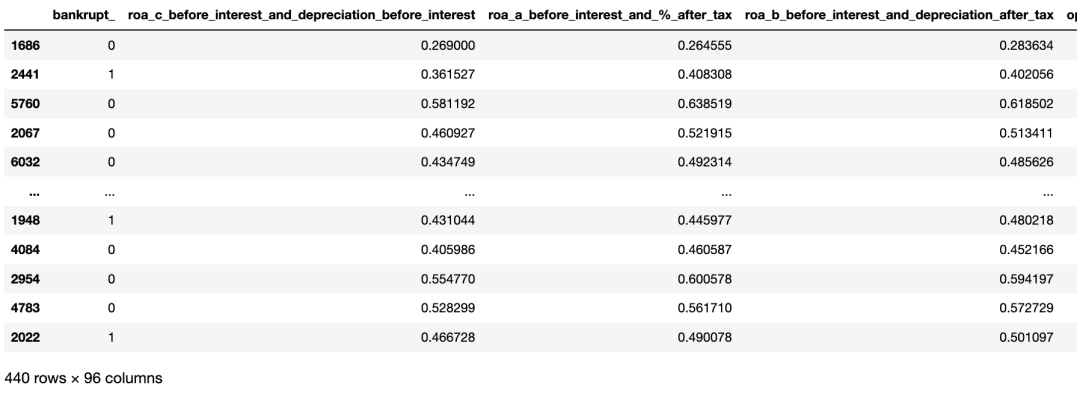
3.3 下采样
首先对数据集进行下采样,目标比例为bankrupt vs non bankrupt = 50 vs 50。
bankruptcy_df2 = bankruptcy_df.sample(frac=1) #Shuffle Bankruptcy df  bankruptcy_df_b = bankruptcy_df2.loc[bankruptcy_df2["bankrupt_"] == 1]
bankruptcy_df_nb = bankruptcy_df2.loc[bankruptcy_df2["bankrupt_"] == 0][:220]  bankruptcy_subdf_comb = pd.concat([bankruptcy_df_b,bankruptcy_df_nb])
bankruptcy_subdf = bankruptcy_subdf_comb.sample(frac=1,random_state=42)  bankruptcy_subdf
再次绘图查看正负样本数。
sns.countplot(bankruptcy_subdf["bankrupt_"])
随机选择220家非破产公司和220家破产公司。
4. 特征工程
bankruptcy_subdf2 = bankruptcy_subdf.drop(["net_income_flag"],axis=1)
bankruptcy_subdf2.shape (440, 95)
4.1 相关矩阵
fig = plt.figure(figsize=(30,20))
ax1 = fig.add_subplot(1,1,1)
sns.heatmap(bankruptcy_subdf2.corr(),ax=ax1,cmap="coolwarm")
4.1.1 找出与破产相关的最高特征
根据对破产企业的基本认识,破产企业资产少、负债高、盈利能力低、现金流少。可以朝这个方向分析我们的数据集。
corr=bankruptcy_subdf2[bankruptcy_subdf2.columns[:-1]].corr()['bankrupt_'][:]  corr_df = pd.DataFrame(corr)  print("Correlations to Bankruptcy:")
for index, row in corr_df["bankrupt_"].iteritems():  if row!=1.0 and row>=0.5:  print(f'Positive Correlation: {index}')  elif row!=1.0 and row<=-0.5:  print(f'Negative Correlation: {index}')
Correlations to Bankruptcy:
Negative Correlation: roa_c_before_interest_and_depreciation_before_interest
Negative Correlation: roa_b_before_interest_and_depreciation_after_tax
Negative Correlation: net_value_per_share_b_
Negative Correlation: net_value_per_share_a_
Negative Correlation: net_value_per_share_c_
Negative Correlation: persistent_eps_in_the_last_four_seasons
Negative Correlation: per_share_net_profit_before_tax_yuan_¥_
Positive Correlation: debt_ratio_%
Negative Correlation: net_worth_assets
Negative Correlation: net_profit_before_tax_paid_in_capital
Negative Correlation: total_income_total_expense
这些特征代表什么
-
roa_c_before_interest_and_depreciation_before_interest息前资产收益率和息前折旧:总资产收益率–如果总资产收益率低,破产风险高
-
roa_a_before_interest_and_after_tax息前和税后利润:总资产回报率–如果总资产回报率较低,破产风险较高
-
roa_b_before_interest_and_depreciation_after_tax利润不计利息及税后折旧:总资产回报率–如果总资产回报率较低,破产风险较高
-
debt_ratio负债率:负债占总资产的比例–价值越高,负债占资产的比例越高,导致破产风险越高
-
net_worth_assets净资产:净资产越少,破产风险越高
-
retained_earnings_to_total_assets留存收益与总资产之比:留存收益越少,破产风险越高
-
total_income_total_expense总费用:收入与费用之比较低,破产风险较高
-
net_income_to_total_assets净收入与总资产之比:净收入越低,破产风险越高
从结果看,导致公司违约风险越高的特征,似乎与背景知识一致。
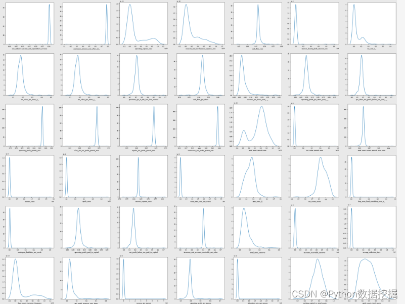
4.2 下采样后特征分布可视化
# Visualisation of distributions after sub-sampling
cols = list(bankruptcy_subdf2.columns)
ncols = 8
nrows = math.ceil(len(cols) / ncols)  fig, ax = plt.subplots(nrows, ncols, figsize = (4.5 * ncols, 4 * nrows))
for i in range(len(cols)):  sns.kdeplot(bankruptcy_subdf2[cols[i]], ax = ax[i // ncols, i % ncols])  if i % ncols != 0:  ax[i // ncols, i % ncols].set_ylabel(" ")
plt.tight_layout()
plt.show()
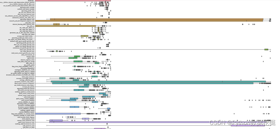
4.3 所有特征的箱线图
plt.figure(figsize=(30,20))
boxplot=sns.boxplot(data=bankruptcy_subdf2,orient="h")
boxplot.set(xscale="log")
plt.show()
4.4 异常值处理
quartile1 = bankruptcy_subdf2.quantile(q=0.25,axis=0)
# display(quartile1)
quartile3 = bankruptcy_subdf2.quantile(q=0.75,axis=0)
# display(quartile3)
IQR = quartile3 -quartile1
lower_limit = quartile1-1.5*IQR
upper_limit = quartile3+1.5*IQR  lower_limit = lower_limit.drop(["bankrupt_"])
upper_limit = upper_limit.drop(["bankrupt_"])
# print(lower_limit)
# print(" ")
# print(upper_limit)  bankruptcy_subdf2_out = bankruptcy_subdf2[((bankruptcy_subdf2<lower_limit) | (bankruptcy_subdf2>upper_limit)).any(axis=1)]
display(bankruptcy_subdf2_out.shape)
display(bankruptcy_subdf2.shape)
(423, 95) (440, 95)
额外复制一份表,供后续分析处理。
bankruptcy_subdf3 = bankruptcy_subdf2_out.copy()
bankruptcy_subdf3
下采样后且去除离群值后的分布可视化。
# Visualisation of distributions after sub-sampling after outlier removal
cols = list(bankruptcy_subdf3.columns)
ncols = 8
nrows = math.ceil(len(cols) / ncols)  fig, ax = plt.subplots(nrows, ncols, figsize = (4.5 * ncols, 4 * nrows))
for i in range(len(cols)):  sns.kdeplot(bankruptcy_subdf3[cols[i]], ax = ax[i // ncols, i % ncols],fill=True,color="red")  sns.kdeplot(bankruptcy_subdf2[cols[i]], ax = ax[i // ncols, i % ncols],color="green")  if i % ncols != 0:  ax[i // ncols, i % ncols].set_ylabel(" ")
plt.tight_layout()
plt.show() 
5 数据预处理
5.1 特征编码
所有类别在基础数据中都已编码完成,因此这里不需要再次编码列。在实际工作中,这一步大概率是必不可少的,编码技术也是尤其重要,需要好好掌握。如果你还不了解或不是很了解,推荐查看:
5.2 Log转换
这一步是为了去除数据中的偏态分布。
# Log transform to remove skews
target = bankruptcy_subdf3['bankrupt_']
bankruptcy_subdf4 = bankruptcy_subdf3.drop(["bankrupt_"],axis=1)  def log_trans(data):  for col in data:  skew = data[col].skew()  if skew>=0.5 or skew<=0.5:  data[col] = np.log1p(data[col])  else:  continue  return data  bankruptcy_subdf4_log = log_trans(bankruptcy_subdf4)
bankruptcy_subdf4_log.head()
5.2.1 Log转换数据的箱线图
plt.figure(figsize=(30,20))
boxplot=sns.boxplot(data=bankruptcy_subdf4_log,orient="h")
boxplot.set(xscale="log")
plt.show()
5.2.2 Log转换后的数据分布可视化
# 在下采样后、去除离群值及log变换后的数据分布的可视化
compare_subdf2 = bankruptcy_subdf2.drop(["bankrupt_"],axis=1)  cols = list(bankruptcy_subdf4.columns)
ncols = 8
nrows = math.ceil(len(cols) / ncols)  fig, ax = plt.subplots(nrows, ncols, figsize = (4.5 * ncols, 4 * nrows))
for i in range(len(cols)):  sns.kdeplot(bankruptcy_subdf4_log[cols[i]], ax = ax[i // ncols, i % ncols],fill=True,color="red")  sns.kdeplot(bankruptcy_subdf2[cols[i]], ax = ax[i // ncols, i % ncols],color="green")  if i % ncols != 0:  ax[i // ncols, i % ncols].set_ylabel(" ")
plt.tight_layout()
plt.show()
print("Red represents distributions after log transforms, green represents before log transform")
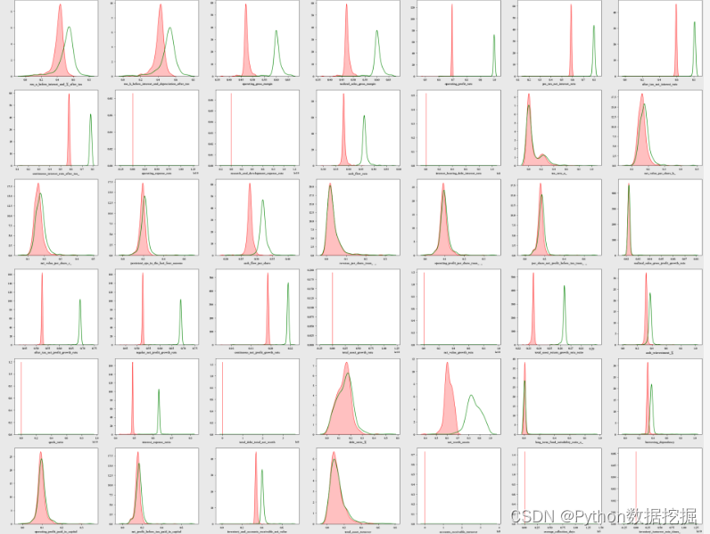
红色表示Log变换后的分布,绿色表示Log变换前的分布。(完整数据集:关注@公众号:数据STUDIO,联系云朵君获取)
6 使用Pycaret构建模型
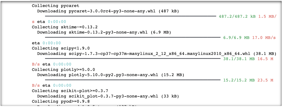
本次模型构建使用的是自动机器学习框架pycaret,如果你还没有安装,可使用下述命令安装即可。
pip install -U --ignore-installed --pre pycaret
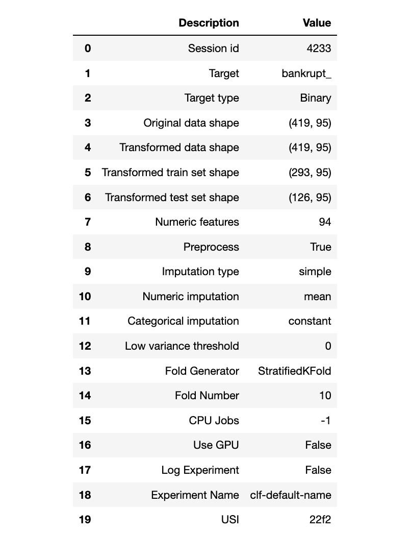
在pycaret中自动完成训练及测试数据的切分工作。
from pycaret.classification import *
exp_name = setup(data = bankruptcy_subdf4,  target = bankruptcy_subdf3["bankrupt_"])
compare_models()
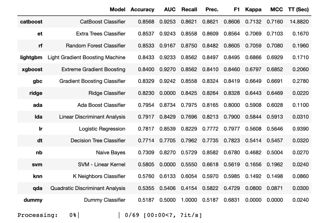
Pycaret显示,3种模型的准确性最高的是
-
LightGBM分类器
-
梯度提升GBC分类器
-
XGBoost分类器
接下来将使用这5个模型进行超参数调优。
6.1 选定模型交叉验证
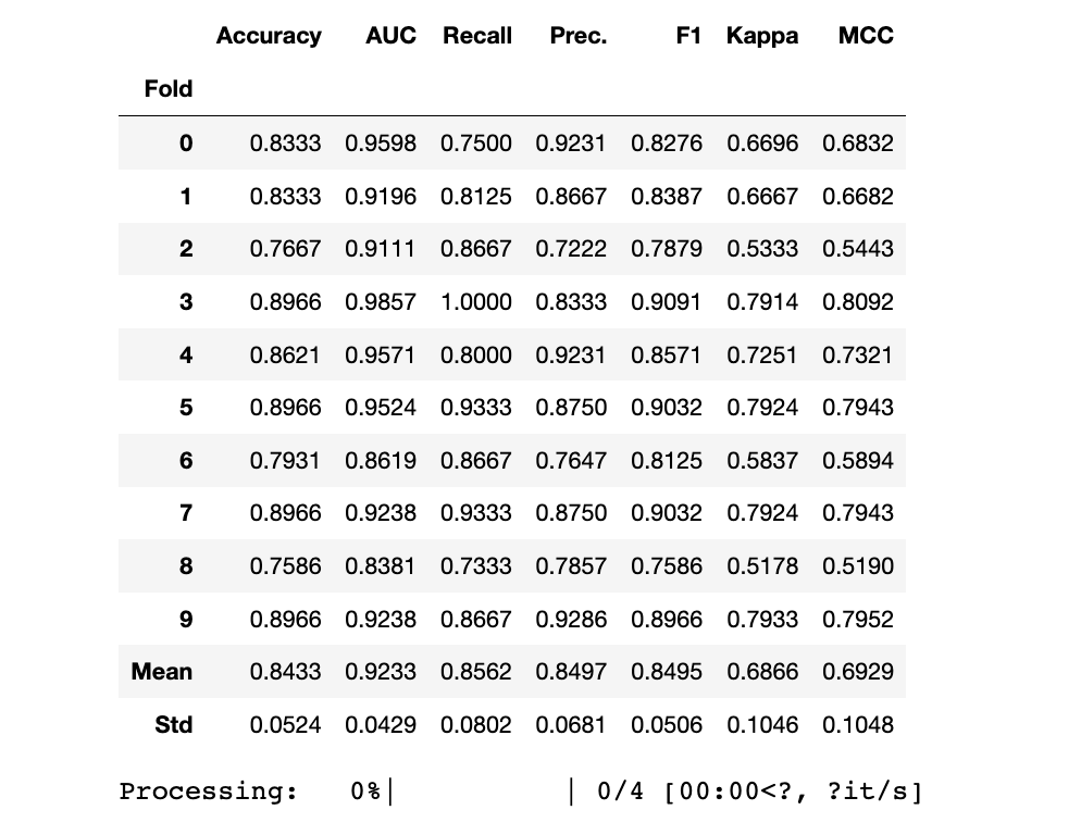
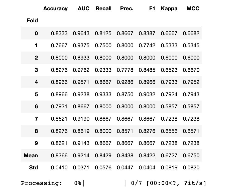
LightGBM
print("LGBM Model")
lgb_clf = create_model("lightgbm")
lgb_clf_scoregrid = pull()
LGBM Model
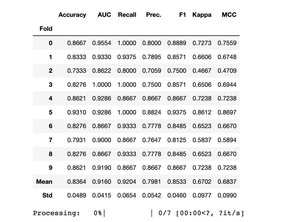
GBC
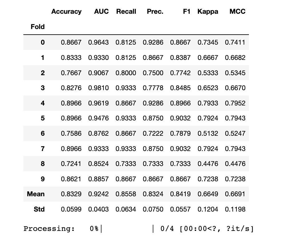
print("GBC Model")
gbc_clf = create_model("gbc")
gbc_clf_scoregrid = pull()
GBC Model
XGBoost
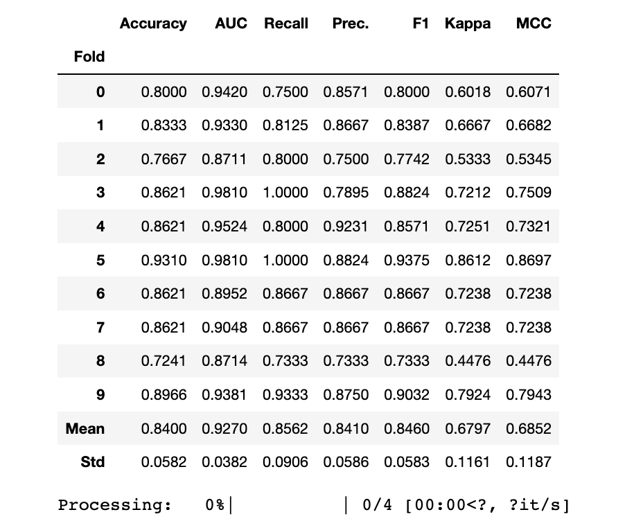
print("XGB Model")
xgb_clf = create_model("xgboost")
xgb_clf_scoregrid = pull()
XGB Model
7 使用Pycaret进行超参数调优
7.1 模型调优
LightGBM
print("Before Tuning")
print(lgb_clf_scoregrid.loc[["Mean","Std"]])
print("")
lgb_clf = tune_model(lgb_clf,choose_better=True)
print(lgb_clf)
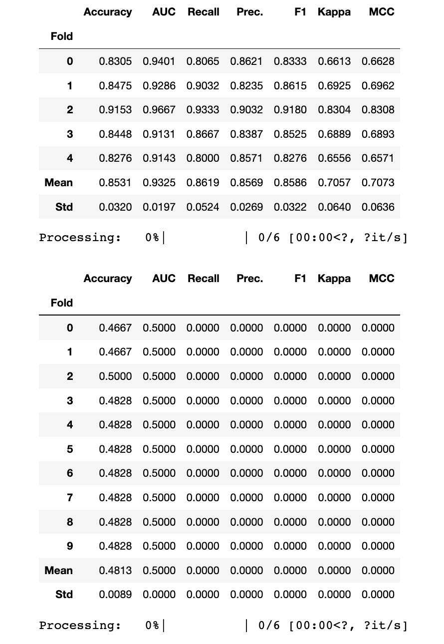
Before Tuning  Accuracy     AUC  Recall   Prec.      F1   Kappa     MCC
Fold
Mean    0.8433  0.9233  0.8562  0.8497  0.8495  0.6866  0.6929
Std     0.0524  0.0429  0.0802  0.0681  0.0506  0.1046  0.1048
GBC
print("Before Tuning")
print(gbc_clf_scoregrid.loc[["Mean","Std"]])
print("")
gbc_clf = tune_model(gbc_clf,choose_better=True)
print(gbc_clf)
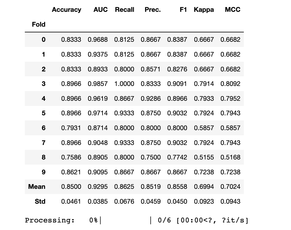
Before Tuning  Accuracy     AUC  Recall   Prec.      F1   Kappa     MCC
Fold
Mean    0.8329  0.9242  0.8558  0.8324  0.8419  0.6649  0.6691
Std     0.0599  0.0403  0.0634  0.0750  0.0557  0.1204  0.1198
XGBoost
print("Before Tuning")
print(xgb_clf_scoregrid.loc[["Mean","Std"]])
print("")
xgb_clf = tune_model(xgb_clf,choose_better = True)
print(xgb_clf)
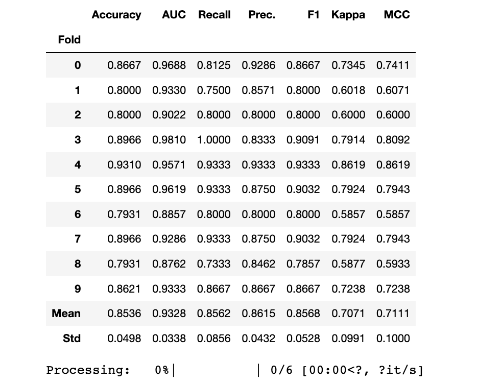
Before Tuning  Accuracy     AUC  Recall   Prec.      F1   Kappa     MCC
Fold
Mean    0.8400  0.9270  0.8562  0.8410  0.8460  0.6797  0.6852
Std     0.0582  0.0382  0.0906  0.0586  0.0583  0.1161  0.1187
7.2 模型集成
-
Bagged & Boosting 方法
-
Blending
-
Stacking
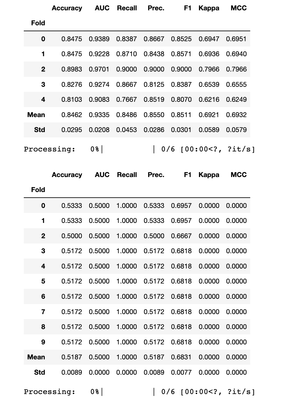
LightGBM
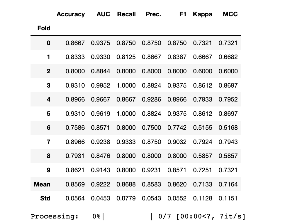
# Original
print(lgb_clf_scoregrid.loc[['Mean', 'Std']])  # Compare the original against bagged and boosted  # Bagged
lgb_clf = ensemble_model(lgb_clf,fold =5,choose_better = True)
# Boosted
lgb_clf = ensemble_model(lgb_clf,method="Boosting",choose_better = True)
      Accuracy     AUC  Recall   Prec.      F1   Kappa     MCC
Fold
Mean    0.8433  0.9233  0.8562  0.8497  0.8495  0.6866  0.6929
Std     0.0524  0.0429  0.0802  0.0681  0.0506  0.1046  0.1048
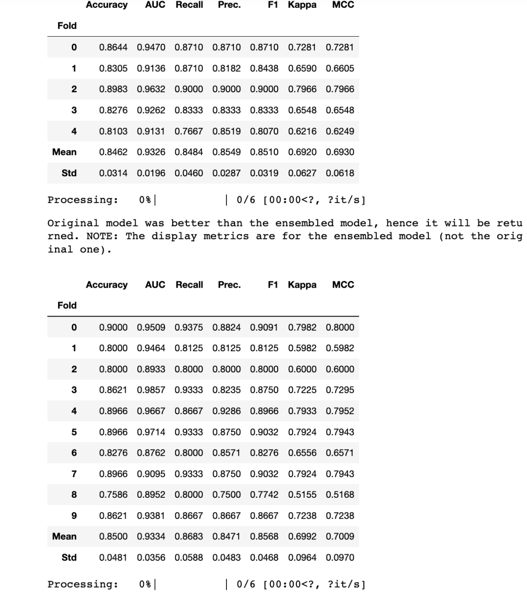
GBC
# Original
print(gbc_clf_scoregrid.loc[['Mean', 'Std']])  # Compare the original against bagged and boosted  # Bagged
gbc_clf = ensemble_model(gbc_clf,fold =5,choose_better = True)
# Boosted
gbc_clf = ensemble_model(gbc_clf,method="Boosting",choose_better = True)
      Accuracy     AUC  Recall   Prec.      F1   Kappa     MCC
Fold
Mean    0.8329  0.9242  0.8558  0.8324  0.8419  0.6649  0.6691
Std     0.0599  0.0403  0.0634  0.0750  0.0557  0.1204  0.1198
XGBoost
# Original
print(xgb_clf_scoregrid.loc[['Mean', 'Std']])  # Compare the original and boosted against bagged and boosted  # Bagged
xgb_clf = ensemble_model(xgb_clf,fold =5,choose_better = True)
# Boosted
xgb_clf = ensemble_model(xgb_clf,method="Boosting",choose_better = True)
      Accuracy     AUC  Recall   Prec.      F1   Kappa     MCC
Fold
Mean    0.8400  0.9270  0.8562  0.8410  0.8460  0.6797  0.6852
Std     0.0582  0.0382  0.0906  0.0586  0.0583  0.1161  0.1187
7.3.1 Blend Models
blend_models([lgb_clf, gbc_clf, xgb_clf],choose_better=True)
7.3.2 Stacking
stacker = stack_models(lgb_clf,gbc_clf) #remove xgb as some issues
print(stacker)
8 模型评估
# evaluate_model(lgb_clf)
# evaluate_model(gbc_clf)
# evaluate_model(xgb_clf)
8.1 ROC-AUC
plot_model(stacker, plot = 'auc')
# Stacked classifier from ensembling
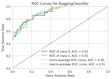
plot_model(lgb_clf, plot = 'auc')
# lgb最适合Bagging集成并被选中
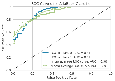
plot_model(gbc_clf, plot = 'auc')
# gbc最适合Boosting集成并被选中
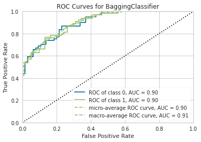
plot_model(xgb_clf, plot = 'auc')
# 基本的xgb分类器在经过调优和集成后仍然表现最好,因此选择了它 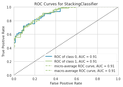
8.2 混淆矩阵
plot_model(stacker,   plot = 'confusion_matrix',   plot_kwargs = {'percent' : True})
plot_model(lgb_clf,   plot = 'confusion_matrix',   plot_kwargs = {'percent' : True})
plot_model(gbc_clf,   plot = 'confusion_matrix',   plot_kwargs = {'percent' : True})
plot_model(xgb_clf, plot = 'confusion_matrix', plot_kwargs = {'percent' : True}) 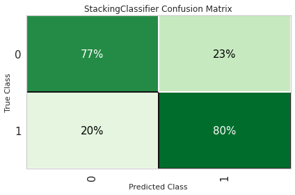


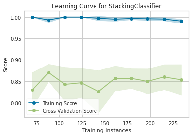
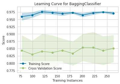
8.3 学习曲线
plot_model(stacker, plot = 'learning')
plot_model(lgb_clf, plot = 'learning')
就到这里了!
相关文章:
企业级实战项目:基于 pycaret 自动化预测公司是否破产
本文系数据挖掘实战系列文章,我跟大家分享一个数据挖掘实战,与以往的数据实战不同的是,用自动机器学习方法完成模型构建与调优部分工作,深入理解由此带来的便利与效果。 1. Introduction 本文是一篇数据挖掘实战案例,…...
dl转置卷积
转置卷积 转置卷积,顾名思义,通过名字我们应该就能看出来,其作用和卷积相反,它可以使得图像的像素增多 上图的意思是,输入是22的图像,卷积核为22的矩阵,然后变换成3*3的矩阵 代码如下 import…...

详解结构体(包含结构体内存对齐,柔性数组,位段)【尊嘟很详细】
结构体 结构体是一些值的集合,这些值称为成员变量,结构的成员可以是标量、数组、指针,甚至是其他结构体。 成员名可以与程序中其它变量同名,互不干扰。 结构体的定义 (struct结构名{}) struct books {int a;c…...

我的NPI项目之Android系统升级 - 同平台多产品的OTA
因为公司业务中涉及的面比较广泛,虽然都是提供移动终端PDA,但是使用的场景很多时候是不同的。例如,有提供给大型物流仓储的设备,对这样的设备必需具备扫码功能,键盘(戴手套操作),耐用…...

pnpm包管理器
官网 优点 快速 pnpm 比 npm 快了近 2 倍高效 node_modules 中的所有文件均克隆或硬链接自单一存储位置支持单体仓库 pnpm 内置了对单个源码仓库中包含多个软件包的支持权限严格 pnpm 创建的 node_modules 默认并非扁平结构,因此代码无法对任意软件包进行访问 安…...

flutter websocket发送ping包?
背景 服务端要求flutter客户端隔一段时间发送ping包,以此来建立心跳管理长连接。 代码 import package:web_socket_channel/io.dart; IOWebSocketChannel _channel IOWebSocketChannel.connect(Uri.parse(SocketService.url),pingInterval: const Duration(seco…...
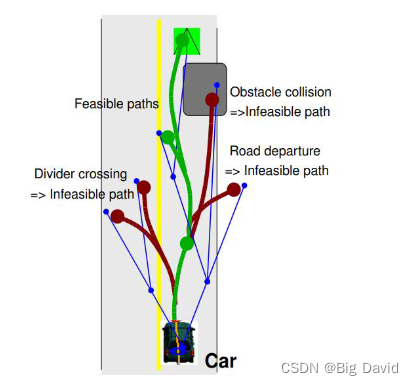
基于采样的自动驾驶规划算法 - PRM,RRT,RRT*,CL-RRT
本文将讲解PRM,RRT,RRT*自动驾驶规划算法原理,不正之处望读者指正 0 前言 机器人运动规划的基本任务:从开始位置到目标位置的运动 (1)如何躲避构型空间出现的障碍物 (2)如何满足机器…...
CGAL的D维范围树和线段树
范围树和线段树是两种数据结构,用于高效地处理和查询数据。 范围树(Range Tree)是一种二叉树,它通过递归地将每个节点分割成两个子节点来存储一个点集。每个节点表示一个范围,并且存储该范围内所有点的最小和最大值。范…...
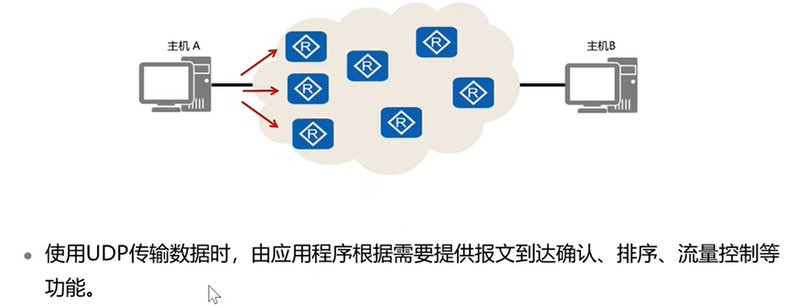
005.HCIA 传输层
传输层定义了主机应用程序之间端到端的连通性。传输层中最为常见的两个协议分别是传输控制协议TCP (Transmission Control Protocol)和用户数据包协议UDP (User Datagram Protocol)。 1、相关概念 a. 传输层的端口 端口范围:0-65535 知名端口:0-1023&…...
LLM之RAG实战(八)| 使用Neo4j和LlamaIndex实现多模态RAG
人工智能和大型语言模型领域正在迅速发展。一年前,没有人使用LLM来提高生产力。时至今日,很难想象我们大多数人或多或少都在使用LLM提供服务,从个人助手到文生图场景。由于大量的研究和兴趣,LLM每天都在变得越来越好、越来越聪明。…...
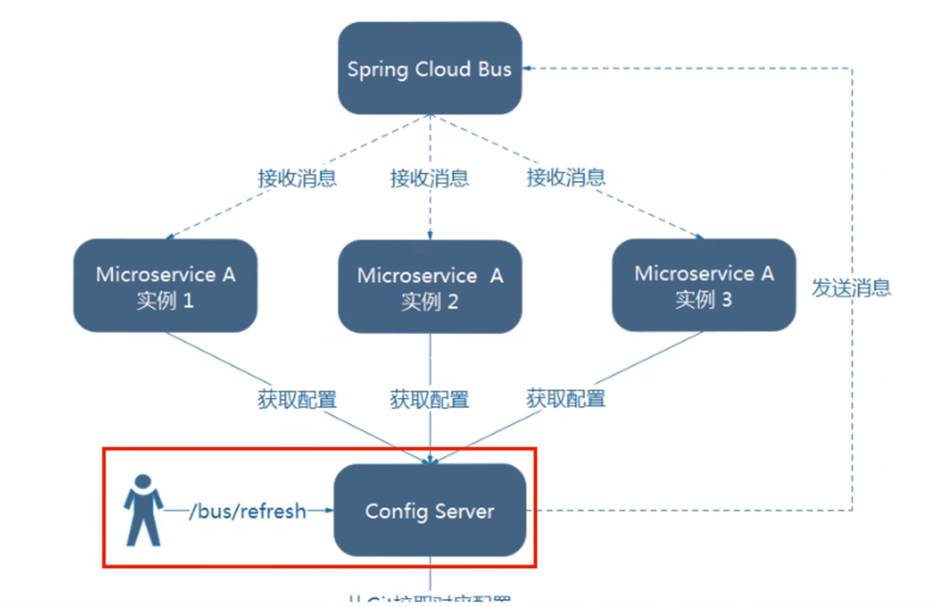
【SpringCloud笔记】(10)消息总线之Bus
Bus 前言 戳我了解Config 学习Config中我们遇到了一个问题: 当我们修改了GitHub上配置文件内容,微服务需要配置动态刷新并且需要手动向客户端发送post请求刷新微服务之后才能获取到GitHub修改过后的内容 假如有多个微服务客户端3355/3366/3377…等等…...

超酷的爬虫可视化界面
大家好,本文主要介绍使用tkinter获取本地文件夹、设置文本、创建按钮下拉框和对界面进行布局。 1.导入tkinter库 导入tkinter的库,可以使用ttkbootstrap美化生成的界面 ttkbootstrap官网地址:https://ttkbootstrap.readthedocs.io/en/late…...

【kafka消息里会有乱序消费的情况吗?如果有,是怎么解决的?】
文章目录 什么是消息乱序消费了?顺序生产,顺序存储,顺序消费如何解决乱序数据库乐观锁是怎么解决这个乱序问题吗 保证消息顺序消费两种方案固定分区方案乐观锁实现方案 前几天刷着视频看见评论区有大佬问了这个问题:你们的kafka消…...

【PID精讲12】基于MATLAB和Simulink的仿真教程
文章目录 写在前面一、基于Simulink的仿真1. 新建Simulink模型2. 保存Simulink模型3. 建模4. 运行二、基于MATLAB的仿真1. 编码2. 运行3. 调整曲线格式4. 导出图窗写在前面 第11讲介绍的连续系统的数字PID仿真是基于 Matlab的 M 语言实现的,对于初学者或者工程应用人员来说,…...

手机无人直播:解放直播的新方式
现如今,随着科技的迅猛发展,手机已经成为我们生活中不可或缺的一部分。除了通讯、娱乐等功能外,手机还能够通过直播功能将我们的生活实时分享给他人。而针对传统的直播方式,使用手机进行无人直播成为了一种全新的选择。 手机无人…...
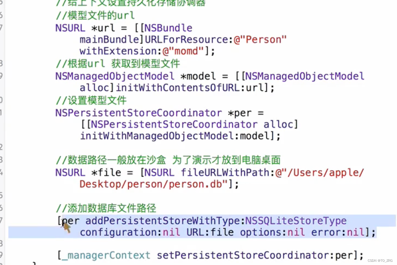
ios 之 数据库、地理位置、应用内跳转、推送、制作静态库、CoreData
第一节:数据库 常见的API SQLite提供了一系列的API函数,用于执行各种数据库相关的操作。以下是一些常用的SQLite API函数及其简要说明:1. sqlite3_initialize:- 初始化SQLite库。通常在开始使用SQLite之前调用,但如果没有调用&a…...

Django(三)
1.快速上手 确保app已注册 【settings.py】 编写URL和视图函数对应关系 【urls.py】 编写视图函数 【views.py】 启动django项目 命令行启动python manage.py runserverPycharm启动 1.1 再写一个页面 2. templates模板 2.1 静态文件 2.1.1 static目录 2.1.2 引用静态…...

vscode括号颜色突然变成白色的了,怎么解决
更新版本后发现vscode的各种括号都变成了白色,由于分色括号已经使用习惯,突然变成白色非常不舒服,尝试多次后,为大家提供一下几种解决方式,希望能帮到同样受到此种困惑的你: 第一种: 首先打开…...

测试服务器带宽(ubuntu)
apt install python3 python3-pippip3 install speedtest-clispeestest-cli...

【WPF】使用Behavior以及ValidationRule实现表单校验
文章目录 使用ValidationRule实现检测用户输入EmptyValidationRule 非空校验TextBox设置非空校验TextBox设置非空校验并显示校验提示 结语 使用ValidationRule实现检测用户输入 EmptyValidationRule是TextBox内容是否为空校验,TextBox的Binding属性设置ValidationRu…...

在HarmonyOS ArkTS ArkUI-X 5.0及以上版本中,手势开发全攻略:
在 HarmonyOS 应用开发中,手势交互是连接用户与设备的核心纽带。ArkTS 框架提供了丰富的手势处理能力,既支持点击、长按、拖拽等基础单一手势的精细控制,也能通过多种绑定策略解决父子组件的手势竞争问题。本文将结合官方开发文档,…...

连锁超市冷库节能解决方案:如何实现超市降本增效
在连锁超市冷库运营中,高能耗、设备损耗快、人工管理低效等问题长期困扰企业。御控冷库节能解决方案通过智能控制化霜、按需化霜、实时监控、故障诊断、自动预警、远程控制开关六大核心技术,实现年省电费15%-60%,且不改动原有装备、安装快捷、…...

电脑插入多块移动硬盘后经常出现卡顿和蓝屏
当电脑在插入多块移动硬盘后频繁出现卡顿和蓝屏问题时,可能涉及硬件资源冲突、驱动兼容性、供电不足或系统设置等多方面原因。以下是逐步排查和解决方案: 1. 检查电源供电问题 问题原因:多块移动硬盘同时运行可能导致USB接口供电不足&#x…...

智能分布式爬虫的数据处理流水线优化:基于深度强化学习的数据质量控制
在数字化浪潮席卷全球的今天,数据已成为企业和研究机构的核心资产。智能分布式爬虫作为高效的数据采集工具,在大规模数据获取中发挥着关键作用。然而,传统的数据处理流水线在面对复杂多变的网络环境和海量异构数据时,常出现数据质…...

使用 Streamlit 构建支持主流大模型与 Ollama 的轻量级统一平台
🎯 使用 Streamlit 构建支持主流大模型与 Ollama 的轻量级统一平台 📌 项目背景 随着大语言模型(LLM)的广泛应用,开发者常面临多个挑战: 各大模型(OpenAI、Claude、Gemini、Ollama)接口风格不统一;缺乏一个统一平台进行模型调用与测试;本地模型 Ollama 的集成与前…...

Springboot社区养老保险系统小程序
一、前言 随着我国经济迅速发展,人们对手机的需求越来越大,各种手机软件也都在被广泛应用,但是对于手机进行数据信息管理,对于手机的各种软件也是备受用户的喜爱,社区养老保险系统小程序被用户普遍使用,为方…...

【Java学习笔记】BigInteger 和 BigDecimal 类
BigInteger 和 BigDecimal 类 二者共有的常见方法 方法功能add加subtract减multiply乘divide除 注意点:传参类型必须是类对象 一、BigInteger 1. 作用:适合保存比较大的整型数 2. 使用说明 创建BigInteger对象 传入字符串 3. 代码示例 import j…...
多光源(Multiple Lights))
C++.OpenGL (14/64)多光源(Multiple Lights)
多光源(Multiple Lights) 多光源渲染技术概览 #mermaid-svg-3L5e5gGn76TNh7Lq {font-family:"trebuchet ms",verdana,arial,sans-serif;font-size:16px;fill:#333;}#mermaid-svg-3L5e5gGn76TNh7Lq .error-icon{fill:#552222;}#mermaid-svg-3L5e5gGn76TNh7Lq .erro…...

智能AI电话机器人系统的识别能力现状与发展水平
一、引言 随着人工智能技术的飞速发展,AI电话机器人系统已经从简单的自动应答工具演变为具备复杂交互能力的智能助手。这类系统结合了语音识别、自然语言处理、情感计算和机器学习等多项前沿技术,在客户服务、营销推广、信息查询等领域发挥着越来越重要…...

【Go语言基础【13】】函数、闭包、方法
文章目录 零、概述一、函数基础1、函数基础概念2、参数传递机制3、返回值特性3.1. 多返回值3.2. 命名返回值3.3. 错误处理 二、函数类型与高阶函数1. 函数类型定义2. 高阶函数(函数作为参数、返回值) 三、匿名函数与闭包1. 匿名函数(Lambda函…...