BikeDNA(七)外在分析:OSM 与参考数据的比较1
BikeDNA(七)外在分析:OSM 与参考数据的比较1
该笔记本将提供的参考自行车基础设施数据集与同一区域的 OSM 数据进行所谓的外部质量评估进行比较。 为了运行这部分分析,必须有一个参考数据集可用于比较。
该分析基于将参考数据集与 OSM 进行比较,并突出显示它们的不同之处,包括自行车基础设施在两个数据集中映射的“程度”以及基础设施“如何”映射,从而查明差异 在网络结构中。
所有差异都是针对与 OSM 相关的参考数据计算的,以 OSM 数据为基线。 例如,网络密度的差异是通过计算参考密度减去 OSM 密度来计算的。 因此,正差值(大于0)表示参考值高出多少; 负差值(低于 0)表示参考值低了多少。 因此,如果差异以百分比形式给出,则 OSM 值将被视为总值 (100%)。
虽然分析是基于比较,但它没有对哪个数据集更好做出先验假设。 对于识别出的差异也是如此:BikeDNA 不允许自动得出哪个数据集质量更好的结论,而是要求用户解释发现的差异的含义,例如,不同的特征是否是遗漏错误的结果 或佣金,以及哪个数据集更正确。 然而,许多低值可能表明参考数据的完整性低于 OSM 数据。
目标是确定的差异可用于评估参考数据集和 OSM 数据集的质量,并支持决定应使用哪个数据集进行进一步分析。
外部比较几乎完全基于笔记本 2a 和 2b 的结果,并期望使用先前笔记本中使用的文件路径来存储结果和绘图。 笔记本 1a、2a、1b 和 2b 必须成功运行才能使用此笔记本。 应用概念和指标的详细解释可以在内在分析笔记本(2a 和 2b)中找到。
为了正确解释一些空间数据质量指标,需要对该区域有一定的了解。
# Load libraries, settings and dataimport json
import pickle
import warnings
from collections import Counterimport contextily as cx
import folium
import geopandas as gpd
import matplotlib as mpl
import matplotlib.colors as colors
import matplotlib.pyplot as plt
import numpy as np
import osmnx as ox
import pandas as pd
import yaml
from matplotlib import cm
from collections import Counterfrom src import evaluation_functions as eval_func
from src import graph_functions as graph_func
from src import plotting_functions as plot_func# Read in dictionaries with settings
%run ../settings/yaml_variables.py
%run ../settings/plotting.py
%run ../settings/tiledict.py
%run ../settings/df_styler.py# Load data
%run ../settings/load_osmdata.py
%run ../settings/load_refdata.py
%run ../settings/load_results.pywarnings.filterwarnings("ignore")
d:\work\miniconda3\envs\bikeDNA\Lib\site-packages\tqdm\auto.py:21: TqdmWarning: IProgress not found. Please update jupyter and ipywidgets. See https://ipywidgets.readthedocs.io/en/stable/user_install.htmlfrom .autonotebook import tqdm as notebook_tqdm
D:\tmp_resource\BikeDNA-main\BikeDNA-main\scripts\settings\plotting.py:49: MatplotlibDeprecationWarning: The get_cmap function was deprecated in Matplotlib 3.7 and will be removed two minor releases later. Use ``matplotlib.colormaps[name]`` or ``matplotlib.colormaps.get_cmap(obj)`` instead.cmap = cm.get_cmap(cmap_name, n)
D:\tmp_resource\BikeDNA-main\BikeDNA-main\scripts\settings\plotting.py:46: MatplotlibDeprecationWarning: The get_cmap function was deprecated in Matplotlib 3.7 and will be removed two minor releases later. Use ``matplotlib.colormaps[name]`` or ``matplotlib.colormaps.get_cmap(obj)`` instead.cmap = cm.get_cmap(cmap_name)
<string>:49: MatplotlibDeprecationWarning: The get_cmap function was deprecated in Matplotlib 3.7 and will be removed two minor releases later. Use ``matplotlib.colormaps[name]`` or ``matplotlib.colormaps.get_cmap(obj)`` instead.
<string>:46: MatplotlibDeprecationWarning: The get_cmap function was deprecated in Matplotlib 3.7 and will be removed two minor releases later. Use ``matplotlib.colormaps[name]`` or ``matplotlib.colormaps.get_cmap(obj)`` instead.OSM graphs loaded successfully!
OSM data loaded successfully!
Reference graphs loaded successfully!
Reference data loaded successfully!
Results from intrinsic analyses loaded successfully!
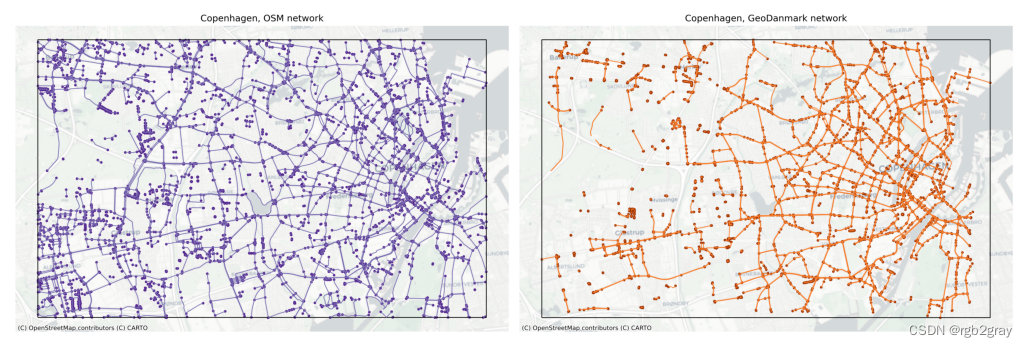
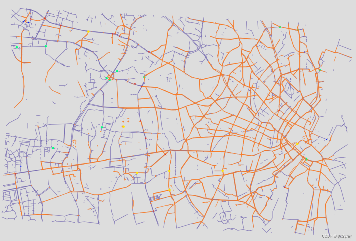
OSM versus reference network
plot_func.plot_saved_maps([osm_results_static_maps_fp + "area_network_osm",ref_results_static_maps_fp + "area_network_reference",]
)
1.数据完整性
本节从数据完整性方面比较 OSM 和参考数据集。 目标是确定一个数据集是否比另一个数据集映射了更多的自行车基础设施,如果是,这些差异是否集中在某些区域。
本节首先比较两个数据集中基础设施的总长度。 然后,首先在全局(研究区域)和局部(网格单元)级别比较基础设施、节点和悬空节点密度(即每平方公里基础设施/节点的长度)。 最后,分别比较受保护和未受保护的自行车基础设施的密度差异。
计算网格局部密度差异作为数据质量的度量也已被例如应用。 Haklay (2010)。
方法
为了考虑自行车基础设施映射方式的差异,网络长度和密度的计算基于基础设施长度,而不是网络边缘的几何长度。 例如,一条 100 米长的双向路径(几何长度:100m)贡献了 200 米的自行车基础设施(基础设施长度:200m)。
解释
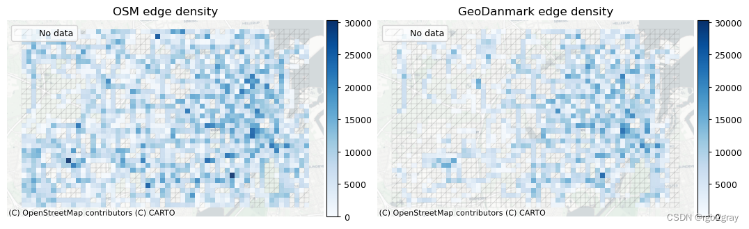
密度差异可能表明数据不完整。 例如,如果网格单元在 OSM 中的边缘密度明显高于参考数据集中的边缘密度,则这可能表明参考数据集中未映射、缺失的特征,或者街道在 OSM 中被错误地标记为自行车基础设施。
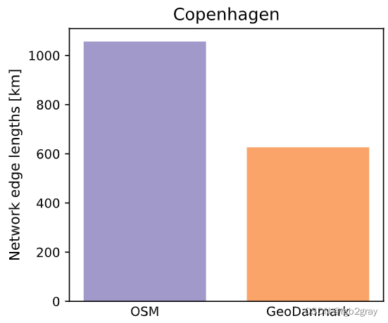
1.1 网络长度
plot_func.compare_print_network_length(osm_edges_simplified.infrastructure_length.sum(),ref_edges_simplified.infrastructure_length.sum(),
)
Length of the OSM data set: 1056.49 km
Length of the reference data set: 626.48 kmThe reference data set is 430.01 km shorter than the OSM data set.
The reference data set is 40.70% shorter than the OSM data set.
# Plot length comparisonset_renderer(renderer_plot)bar_labels = ["OSM", reference_name]
x_positions = [1, 2]
bar_colors = [pdict["osm_base"], pdict["ref_base"]]# Infrastructure length density
data = [osm_edges_simplified.infrastructure_length.sum()/1000,ref_edges_simplified.infrastructure_length.sum()/1000]
y_label = "Network edge lengths [km]"
filepath = compare_results_plots_fp + "network_length_compare"
title = area_nameplot = plot_func.make_bar_plot(data=data,bar_labels=bar_labels,y_label=y_label,x_positions=x_positions,title=title,bar_colors=bar_colors,filepath=filepath,figsize=pdict["fsbar_small"]
)
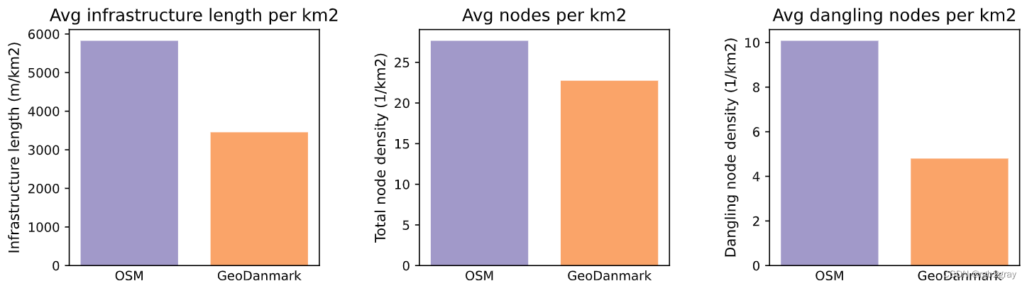
1.2 网络密度
全球网络密度
plot_func.print_network_densities(osm_intrinsic_results, "OSM")
plot_func.print_network_densities(ref_intrinsic_results, "reference")
In the OSM data, there are:- 5824.58 meters of cycling infrastructure per km2.- 27.65 nodes in the cycling network per km2.- 10.08 dangling nodes in the cycling network per km2.In the reference data, there are:- 3453.85 meters of cycling infrastructure per km2.- 22.74 nodes in the cycling network per km2.- 4.80 dangling nodes in the cycling network per km2.
全球网络密度(每平方公里)
# Plot global differenceset_renderer(renderer_plot)# Infrastructure length density
subplotdata = [(osm_intrinsic_results["network_density"]["edge_density_m_sqkm"],ref_intrinsic_results["network_density"]["edge_density_m_sqkm"],),(osm_intrinsic_results["network_density"]["node_density_count_sqkm"],ref_intrinsic_results["network_density"]["node_density_count_sqkm"],),(osm_intrinsic_results["network_density"]["dangling_node_density_count_sqkm"],ref_intrinsic_results["network_density"]["dangling_node_density_count_sqkm"],),
]
subplotx_positions = [[1,2] for j in range(3)]
subplotbar_labels = ["Infrastructure length (m/km2)","Total node density (1/km2)","Dangling node density (1/km2)",
]
filepath = compare_results_plots_fp + "network_densities_compare"
subplottitle = ["Avg infrastructure length per km2","Avg nodes per km2","Avg dangling nodes per km2",
]plot = plot_func.make_bar_subplots(subplot_data=subplotdata,nrows=1,ncols=3,bar_labels=[["OSM", reference_name] for j in range(3)],y_label=subplotbar_labels,x_positions=subplotx_positions,title=subplottitle,bar_colors=[pdict["osm_base"], pdict["ref_base"]],filepath=filepath,wspace=0.4
)
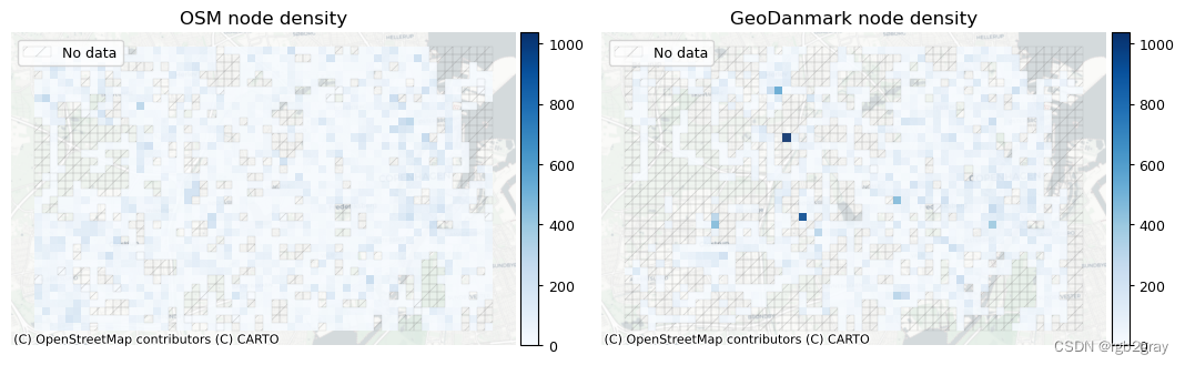
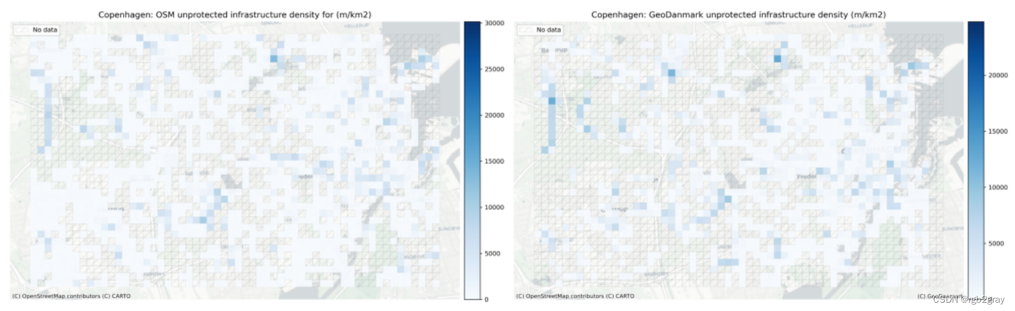
本地网络密度
### Plot density comparisonsset_renderer(renderer_map)# Edge density
plot_cols = ["osm_edge_density", "ref_edge_density"]
plot_func.plot_multiple_grid_results(grid=grid,plot_cols=plot_cols,plot_titles=["OSM edge density", f"{reference_name} edge density"],filepath=compare_results_static_maps_fp + "density_edge_compare",cmap=pdict["pos"],alpha=pdict["alpha_grid"],cx_tile=cx_tile_2,no_data_cols=["count_osm_edges", "count_ref_edges"],use_norm=True,norm_min=0,norm_max = max(grid[plot_cols].max()),figsize = pdict["fsmap"],legend = False,
)# Node density
plot_cols = ["osm_node_density", "ref_node_density"]
plot_func.plot_multiple_grid_results(grid=grid,plot_cols=plot_cols,plot_titles=["OSM node density", f"{reference_name} node density"],filepath=compare_results_static_maps_fp + "density_node_compare",cmap=pdict["pos"],alpha=pdict["alpha_grid"],cx_tile=cx_tile_2,no_data_cols=["count_osm_nodes", "count_ref_nodes"],use_norm=True,norm_min=0,norm_max = max(grid[plot_cols].max()),figsize = pdict["fsmap"],legend = False,
)# Dangling node density
plot_cols = ["osm_dangling_node_density", "ref_dangling_node_density"]
plot_func.plot_multiple_grid_results(grid=grid,plot_cols=plot_cols,plot_titles=["OSM dangling node density", f"{reference_name} dangling node density"],filepath=compare_results_static_maps_fp + "density_danglingnode_compare",cmap=pdict["pos"],alpha=pdict["alpha_grid"],cx_tile=cx_tile_2,no_data_cols=["count_osm_nodes", "count_ref_nodes"],use_norm=True,norm_min=0,norm_max = max(grid[plot_cols].max()),figsize = pdict["fsmap"],legend = False,
)

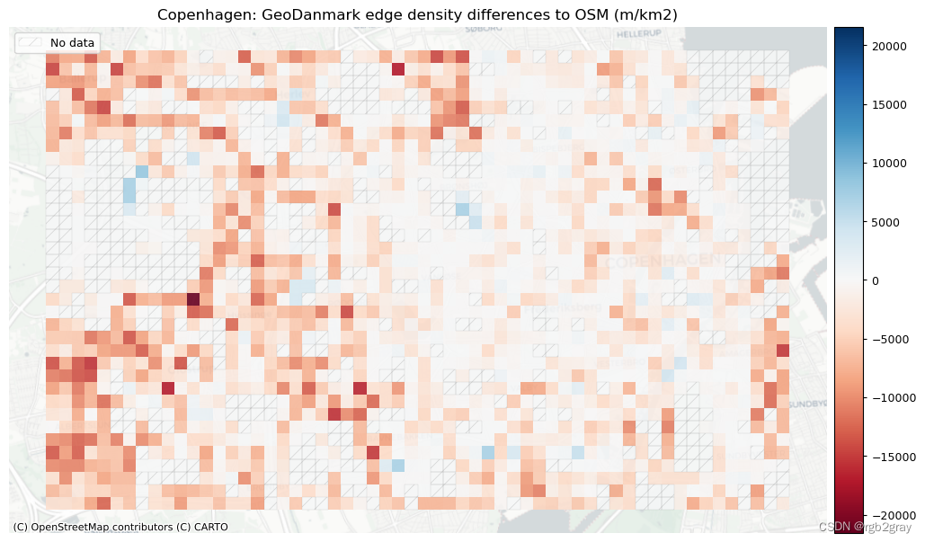
网络密度的局部差异
以OSM数据中的密度作为比较基线,绝对差值计算为“参考值”-“OSM值”。 因此,正值表示基础设施类型的参考密度高于 OSM 密度; 负值表示参考密度低于 OSM 密度。
grid["edge_density_diff"] = grid.ref_edge_density.fillna(0
) - grid.osm_edge_density.fillna(0)grid["node_density_diff"] = grid.ref_node_density.fillna(0
) - grid.osm_node_density.fillna(0)grid["dangling_node_density_diff"] = grid.ref_dangling_node_density.fillna(0
) - grid.osm_dangling_node_density.fillna(0)
# Network density grid plotsset_renderer(renderer_map)plot_cols = ["edge_density_diff", "node_density_diff", "dangling_node_density_diff"]
plot_titles = [area_name + f": {reference_name} edge density differences to OSM (m/km2)",area_name + f": {reference_name} node density differences to OSM (m/km2)",area_name + f": {reference_name} dangling node density differences to OSM (m/km2)"
]
filepaths = [compare_results_static_maps_fp + "edge_density_compare",compare_results_static_maps_fp + "node_density_compare",compare_results_static_maps_fp + "dangling_node_density_compare",
]cmaps = [pdict["diff"]] * 3# Cols for no-data plots
no_data_cols = [("osm_edge_density", "ref_edge_density"),("osm_node_density", "ref_node_density"),("osm_dangling_node_density", "ref_dangling_node_density"),
]cblim_edge = max(abs(min(grid["edge_density_diff"].fillna(value=0))),max(grid["edge_density_diff"].fillna(value=0)),
)cblim_node = max(abs(min(grid["node_density_diff"].fillna(value=0))),max(grid["node_density_diff"].fillna(value=0)),
)cblim_d_node = max(abs(min(grid["dangling_node_density_diff"].fillna(value=0))),max(grid["dangling_node_density_diff"].fillna(value=0)),
)norm_min = [-cblim_edge, -cblim_node, -cblim_d_node]
norm_max = [cblim_edge, cblim_node, cblim_d_node]plot_func.plot_grid_results(grid=grid,plot_cols=plot_cols,plot_titles=plot_titles,filepaths=filepaths,cmaps=cmaps,alpha=pdict["alpha_grid"],cx_tile=cx_tile_2,no_data_cols=no_data_cols,use_norm=True,norm_min=norm_min,norm_max=norm_max,
)


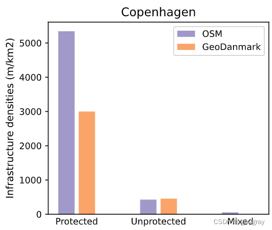
受保护和不受保护的自行车基础设施的密度
受保护/未受保护基础设施的全球网络密度
# Plot global differencesset_renderer(renderer_plot)data_labels = ["protected_density", "unprotected_density", "mixed_density"]
legend_labels = ["OSM", reference_name]
data_osm = [osm_intrinsic_results["network_density"][label + "_m_sqkm"] for label in data_labels
]
data_ref = [ref_intrinsic_results["network_density"][label + "_m_sqkm"] for label in data_labels
]
bar_colors = [pdict["osm_base"], pdict["ref_base"]]
title = f"{area_name}"x_labels = ["Protected", "Unprotected", "Mixed"]
x_axis = [np.arange(len(x_labels)) * 2 - 0.25, np.arange(len(x_labels)) * 2 + 0.25]
x_ticks = np.arange(len(x_labels)) * 2y_label = "Infrastructure densities (m/km2)"filepath = compare_results_plots_fp + "infrastructure_type_density_diff_compare"fig = plot_func.make_bar_plot_side(x_axis=x_axis,data_osm=data_osm,data_ref=data_ref,bar_colors=bar_colors,legend_labels=legend_labels,title=title,x_ticks=x_ticks,x_labels=x_labels,x_label=None,y_label=y_label,filepath=filepath,figsize=pdict["fsbar_small"]
)
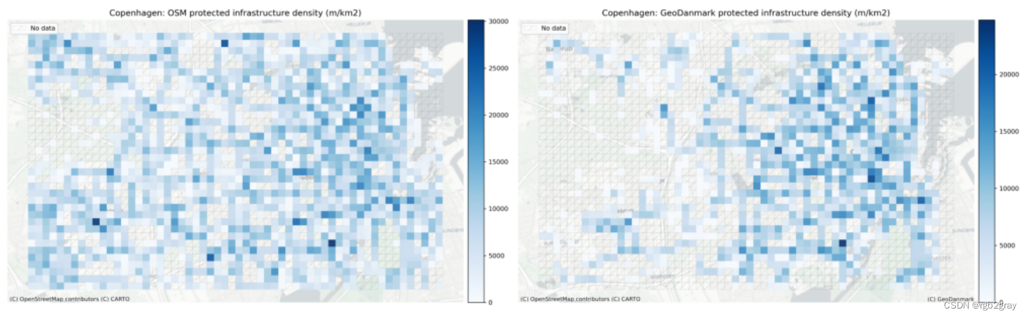
受保护/未受保护基础设施的本地网络密度
if "ref_protected_density" in grid.columns:plot_func.plot_saved_maps([osm_results_static_maps_fp + "density_protected_OSM",ref_results_static_maps_fp + "density_protected_reference",])else:plot_func.plot_saved_maps([osm_results_static_maps_fp + "density_protected_OSM"] * 2, alpha=[1, 0])print(f"No infrastructure is mapped as protected in the {reference_name} data.")if "ref_unprotected_density" in grid.columns:plot_func.plot_saved_maps([osm_results_static_maps_fp + "density_unprotected_OSM",ref_results_static_maps_fp + "density_unprotected_reference",])else:plot_func.plot_saved_maps([osm_results_static_maps_fp + "density_unprotected_OSM"] * 2, alpha=[1, 0])print(f"No infrastructure is mapped as unprotected in the {reference_name} data.")if "ref_mixed_density" in grid.columns:plot_func.plot_saved_maps([osm_results_static_maps_fp + "density_mixed_OSM",ref_results_static_maps_fp + "density_mixed_reference",])else:plot_func.plot_saved_maps([osm_results_static_maps_fp + "density_mixed_OSM"] * 2, alpha=[1, 0])print(f"No infrastructure is mapped as mixed protected/unprotected in the {reference_name} data.")
No infrastructure is mapped as mixed protected/unprotected in the GeoDanmark data.

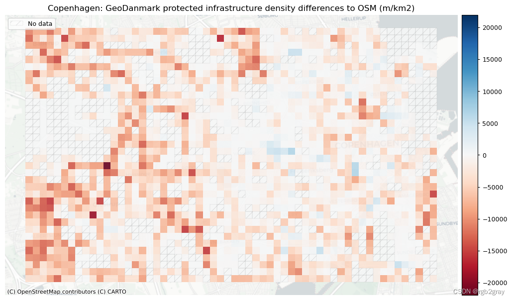
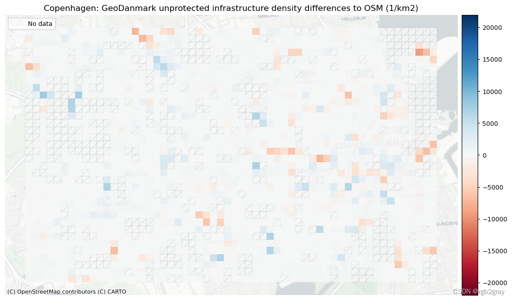
基础设施类型密度的差异
# Computing difference in infrastructure type density# In case no infrastructure with mixed protected/unprotected exist
if "osm_mixed_density" not in grid.columns:grid["osm_mixed_density"] = 0if "ref_mixed_density" not in grid.columns:grid["ref_mixed_density"] = 0if "ref_protected_density" not in grid.columns:grid["ref_protected_density"] = 0if "ref_unprotected_density" not in grid.columns:grid["ref_unprotected_density"] = 0grid["protected_density_diff"] = grid.ref_protected_density.fillna(0
) - grid.osm_protected_density.fillna(0)
grid["unprotected_density_diff"] = grid.ref_unprotected_density.fillna(0
) - grid.osm_unprotected_density.fillna(0)
grid["mixed_density_diff"] = grid.ref_mixed_density.fillna(0
) - grid.osm_mixed_density.fillna(0)
# Infrastructure type density grid plotsset_renderer(renderer_map)plot_cols = ["protected_density_diff", "unprotected_density_diff", "mixed_density_diff"]
plot_cols = [c for c in plot_cols if c in grid.columns]
plot_titles = [area_name + f": {reference_name} protected infrastructure density differences to OSM (m/km2)",area_name + f": {reference_name} unprotected infrastructure density differences to OSM (1/km2)",area_name + f": {reference_name} mixed infrastructure density differences to OSM (1/km2)",
]filepaths = [compare_results_static_maps_fp + "protected_density_compare",compare_results_static_maps_fp + "unprotected_density_compare",compare_results_static_maps_fp + "mixed_density_compare",
]cmaps = [pdict["diff"]] * len(plot_cols)# Cols for no-data plots
no_data_cols = [("osm_edge_density", "ref_edge_density"),("osm_edge_density", "ref_edge_density"),("osm_edge_density", "ref_edge_density"),
]# Create symmetrical color range around zero
cblim = max(abs(min(grid[plot_cols].fillna(value=0).min())),max(grid[plot_cols].fillna(value=0).max()),
)norm_min = [-cblim] * len(plot_cols)
norm_max = [cblim] * len(plot_cols)plot_func.plot_grid_results(grid=grid,plot_cols=plot_cols,plot_titles=plot_titles,filepaths=filepaths,cmaps=cmaps,alpha=pdict["alpha_grid"],cx_tile=cx_tile_2,no_data_cols=no_data_cols,use_norm=True,norm_min=norm_min,norm_max=norm_max,
)

2.网络拓扑结构
在比较数据完整性(即映射了“多少”基础设施)之后,这里我们重点关注网络“拓扑”的差异,它提供了有关“如何”基础设施在两个数据集中映射的信息。 在这里,我们还分析网络边与一个或多个其他边连接的程度,或者它们是否以悬空节点结束。 边缘与相邻边缘正确连接的程度对于可访问性和路由分析等非常重要。
在处理自行车网络上的数据时,首选实际连接的网络元素之间没有间隙的数据集 - 当然反映了真实情况。
识别网络中的悬空节点是识别以“死胡同”结束的边缘的快速且简单的方法。 下冲和过冲分别提供了网络间隙和过度延伸边缘的更精确图像,这给出了悬空节点的误导性计数。
方法
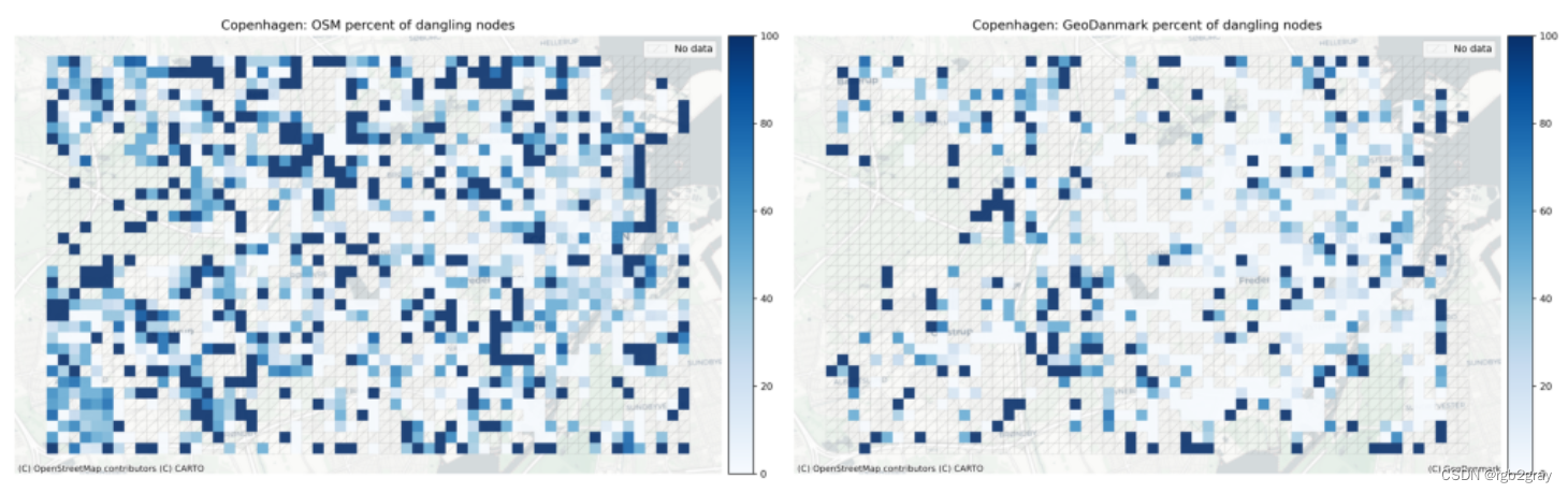
为了识别数据中潜在的间隙或缺失的链接,首先绘制两个数据集中的悬空节点。 然后,单独绘制每个数据集中所有节点中悬挂节点的局部百分比。 最后,我们显示了悬空节点百分比的局部差异。
OSM 和参考数据中的欠调和过调最终会一起绘制在交互式图中,以供进一步检查。
解释
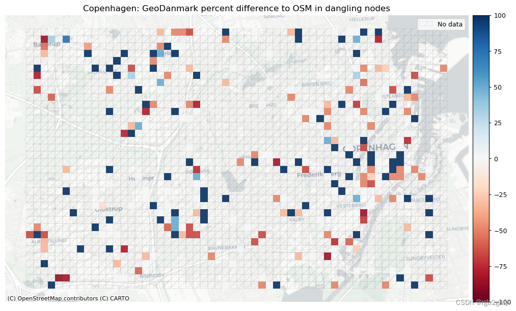
如果一条边在一个数据集中以悬空节点结束,但在另一个数据集中却没有,则表明数据质量存在问题。 数据中缺少连接,或者两条边连接错误。 类似地,悬空节点份额的不同局部率表明自行车网络的映射方式存在差异——尽管在解释中当然应该考虑数据完整性的差异。
下冲是网络数据中误导性差距的明显迹象——尽管它们也可能代表自行车基础设施中的实际差距。 将一个数据集与另一数据集的下冲进行比较可以帮助确定这是数据质量问题还是实际基础设施的质量问题。 交叉口之间存在下冲或间隙的系统差异可能表明不同的数字化策略,因为一些方法会将穿过街道的自行车道绘制为连接的延伸段,而其他方法则会在交叉街道的宽度上引入间隙。 虽然这两种方法都是有效的,但使用前一种方法创建的数据集更适合基于路由的分析。
超调对于分析来说通常不太重要,但大量的超调会引入错误的悬空节点,并扭曲基于节点度或节点与边之间的比率等网络结构的测量。
2.1 简化结果
print(f"Simplifying the OSM network decreased the number of edges by {osm_intrinsic_results['simplification_outcome']['edge_percent_diff']:.1f}%."
)
print(f"Simplifying the OSM network decreased the number of nodes by {osm_intrinsic_results['simplification_outcome']['node_percent_diff']:.1f}%."
)
print("\n")
print(f"Simplifying the {reference_name} network decreased the number of edges by {ref_intrinsic_results['simplification_outcome']['edge_percent_diff']:.1f}%."
)
print(f"Simplifying the {reference_name} network decreased the number of nodes by {ref_intrinsic_results['simplification_outcome']['node_percent_diff']:.1f}%."
)
Simplifying the OSM network decreased the number of edges by 89.0%.
Simplifying the OSM network decreased the number of nodes by 84.4%.Simplifying the GeoDanmark network decreased the number of edges by 91.2%.
Simplifying the GeoDanmark network decreased the number of nodes by 92.2%.
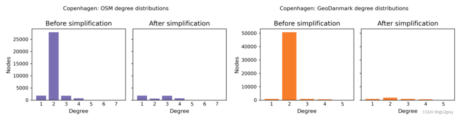
Node degree distribution
degree_sequence_before_osm = sorted((d for n, d in osm_graph.degree()), reverse=True)
degree_sequence_after_osm = sorted((d for n, d in osm_graph_simplified.degree()), reverse=True
)degree_sequence_before_ref = sorted((d for n, d in ref_graph.degree()), reverse=True)
degree_sequence_after_ref = sorted((d for n, d in ref_graph_simplified.degree()), reverse=True
)
# Display already saved degree distribution plotsprint("Note that the two figures below have different y-axis scales.")plot_func.plot_saved_maps([osm_results_plots_fp + "degree_dist_osm",ref_results_plots_fp + "degree_dist_reference"]
)
Note that the two figures below have different y-axis scales.
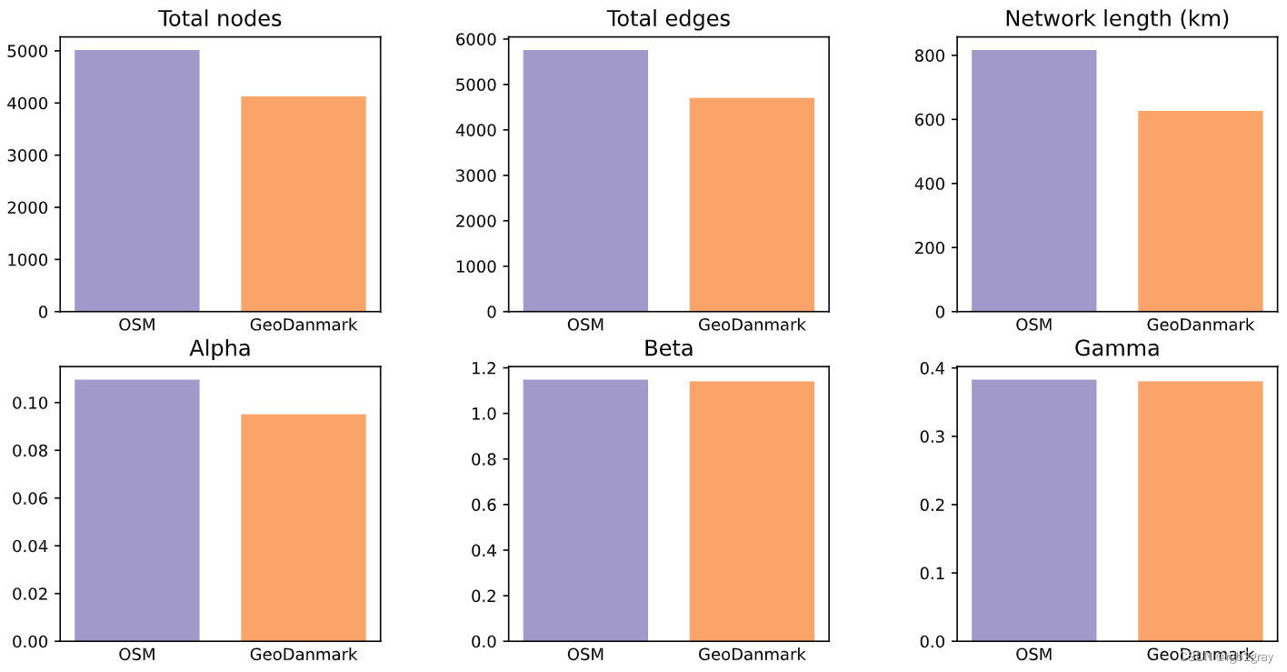
2.2 Alpha、beta 和 gamma 指数
在本小节中,我们计算并对比三个聚合网络指标 alpha、beta 和 gamma。 这些指标通常用于描述网络结构,但作为数据质量的衡量标准,它们仅在与相应数据集的值进行比较时才有意义。 因此,alpha、beta 和 gamma 仅是外在分析的一部分,不包含在内在笔记本中。
虽然无法根据这三个指标中的任何一个本身得出有关数据质量的结论,但对两个数据集的指标进行比较可以表明网络拓扑的差异,从而表明基础设施映射方式的差异。
方法
所有三个索引均使用“eval_func.compute_alpha_beta_gamma”计算。
alpha 值是网络中实际与可能的周期的比率。 网络循环被定义为闭环 - 即在其起始节点上结束的路径。 alpha值的范围是0到1。alpha值为0意味着网络根本没有环,即它是一棵树。 alpha 值为 1 意味着网络完全连接,但这种情况很少见。
beta 值是网络中现有边与现有节点的比率。 beta的取值范围是0到N-1,其中N是现有节点的数量。 beta值为0意味着网络没有边; Beta 值为 N-1 意味着网络完全连接(另请参见 gamma 值 1)。 beta 值越高,在任意一对节点之间可以选择的不同路径(平均)就越多。
gamma 值是网络中现有边与可能边的比率。 连接两个现有网络节点的任何边都被定义为“可能”。 因此,gamma 的取值范围为 0 到 1。gamma 值为 0 表示网络没有边;gamma 值为 0 表示网络没有边; gamma 值为 1 意味着网络的每个节点都连接到每个其他节点。
对于所有三个指数,请参阅 Ducruet 和 Rodrigue,2020。 所有三个指数都可以根据网络连接性进行解释: alpha 值越高,网络中存在的周期越多; beta值越高,路径数量越多,网络复杂度越高; 伽马值越高,任何一对节点之间的边越少。
解释
这些指标并没有过多说明数据质量本身,也对于类似规模的网络的拓扑比较没有用处。 不过,通过比较还是可以得出一些结论。 例如,如果两个网络的索引非常相似,尽管网络例如 具有非常不同的几何长度,这表明数据集是以大致相同的方式映射的,但一个数据集只是比另一个包含更多的特征。 然而,如果网络的总几何长度大致相同,但 alpha、beta 和 gamma 的值不同,则这可能表明两个数据集的结构和拓扑根本不同。
osm_alpha, osm_beta, osm_gamma = eval_func.compute_alpha_beta_gamma(edges=osm_edges_simplified,nodes=osm_nodes_simplified,G=osm_graph_simplified,planar=True,
)  # We assume network to be planar or approximately planarprint(f"Alpha for the simplified OSM network: {osm_alpha:.2f}")
print(f"Beta for the simplified OSM network: {osm_beta:.2f}")
print(f"Gamma for the simplified OSM network: {osm_gamma:.2f}")print("\n")ref_alpha, ref_beta, ref_gamma = eval_func.compute_alpha_beta_gamma(ref_edges_simplified, ref_nodes_simplified, ref_graph_simplified, planar=True
)  # We assume network to be planar or approximately planarprint(f"Alpha for the simplified {reference_name} network: {ref_alpha:.2f}")
print(f"Beta for the simplified {reference_name} network: {ref_beta:.2f}")
print(f"Gamma for the simplified {reference_name} network: {ref_gamma:.2f}")
Alpha for the simplified OSM network: 0.11
Beta for the simplified OSM network: 1.15
Gamma for the simplified OSM network: 0.38Alpha for the simplified GeoDanmark network: 0.10
Beta for the simplified GeoDanmark network: 1.14
Gamma for the simplified GeoDanmark network: 0.38
# Plot alpha, beta, gammaset_renderer(renderer_plot)bar_labels = ["OSM", reference_name]bar_colors = [pdict["osm_base"], pdict["ref_base"]]subplot_data = [(len(osm_nodes_simplified), len(ref_nodes_simplified)),(len(osm_edges_simplified), len(ref_edges_simplified)),(osm_edges_simplified.geometry.length.sum()/1000,ref_edges_simplified.geometry.length.sum()/1000,),(osm_alpha, ref_alpha),(osm_beta, ref_beta),(osm_gamma, ref_gamma),
]
y_label = ["","","","","","",
]
subplottitle = ["Total nodes", "Total edges", "Network length (km)", "Alpha", "Beta", "Gamma"]
filepath = compare_results_plots_fp + "alpha_beta_gamma"plot = plot_func.make_bar_subplots(subplot_data=subplot_data,nrows=2,ncols=3,bar_labels=[["OSM", reference_name] for j in range(6)],y_label=y_label,x_positions=[[1,2] for j in range(6)],title=subplottitle,bar_colors=bar_colors,filepath=filepath,wspace=0.4
);
2.3 悬空节点
osm_dangling_nodes = gpd.read_file(osm_results_data_fp + "dangling_nodes.gpkg")
ref_dangling_nodes = gpd.read_file(ref_results_data_fp + "dangling_nodes.gpkg")
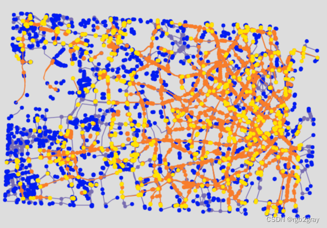
OSM 和参考网络中的悬空节点
# Interactive plot of dangling nodesosm_edges_simplified_folium = plot_func.make_edgefeaturegroup(gdf=osm_edges_simplified,mycolor=pdict["osm_base"],myweight=pdict["line_base"],nametag="OSM edges",show_edges=True,
)osm_nodes_simplified_folium = plot_func.make_nodefeaturegroup(gdf=osm_nodes_simplified,mysize=pdict["mark_base"],mycolor=pdict["osm_base"],nametag="OSM all nodes",show_nodes=True,
)osm_dangling_nodes_folium = plot_func.make_nodefeaturegroup(gdf=osm_dangling_nodes,mysize=pdict["mark_emp"],mycolor=pdict["osm_contrast"],nametag="OSM dangling nodes",show_nodes=True,
)ref_edges_simplified_folium = plot_func.make_edgefeaturegroup(gdf=ref_edges_simplified,mycolor=pdict["ref_base"],myweight=pdict["line_base"],nametag="Reference edges",show_edges=True,
)ref_nodes_simplified_folium = plot_func.make_nodefeaturegroup(gdf=ref_nodes_simplified,mysize=pdict["mark_base"],mycolor=pdict["ref_base"],nametag="Reference all nodes",show_nodes=True,
)ref_dangling_nodes_folium = plot_func.make_nodefeaturegroup(gdf=ref_dangling_nodes,mysize=pdict["mark_emp"],mycolor=pdict["ref_contrast2"],nametag="Reference dangling nodes",show_nodes=True,
)m = plot_func.make_foliumplot(feature_groups=[osm_edges_simplified_folium,osm_nodes_simplified_folium,osm_dangling_nodes_folium,ref_edges_simplified_folium,ref_nodes_simplified_folium,ref_dangling_nodes_folium,],layers_dict=folium_layers,center_gdf=osm_nodes_simplified,center_crs=osm_nodes_simplified.crs,
)bounds = plot_func.compute_folium_bounds(osm_nodes_simplified)
m.fit_bounds(bounds)
m.save(compare_results_inter_maps_fp + "danglingmap_compare.html")display(m)
print("Interactive map saved at " + compare_results_inter_maps_fp.lstrip("../") + "danglingmap_compare.html")
Interactive map saved at results/COMPARE/cph_geodk/maps_interactive/danglingmap_compare.html
悬空节点的局部值
# Compute pct difference relative to OSMgrid["dangling_nodes_diff_pct"] = np.round(100* (grid.count_ref_dangling_nodes - grid.count_osm_dangling_nodes)/ grid.count_osm_dangling_nodes,2,
)
悬空节点占所有节点的百分比
plot_func.plot_saved_maps([osm_results_static_maps_fp + "pct_dangling_nodes_osm",ref_results_static_maps_fp + "pct_dangling_nodes_reference",]
)
悬空节点百分比的局部差异
# Plotset_renderer(renderer_map)# norm color bar
cbnorm_dang_diff = colors.Normalize(vmin=-100, vmax=100)  # from -max to +maxfig, ax = plt.subplots(1, figsize=pdict["fsmap"])
from mpl_toolkits.axes_grid1 import make_axes_locatable
divider = make_axes_locatable(ax)
cax = divider.append_axes("right", size="3.5%", pad="1%")grid.plot(cax=cax,ax=ax,alpha=pdict["alpha_grid"],column="dangling_nodes_diff_pct",cmap=pdict["diff"],legend=True,norm=cbnorm_dang_diff,
)# Add no data patches
grid[grid["dangling_nodes_diff_pct"].isnull()].plot(cax=cax,ax=ax,facecolor=pdict["nodata_face"],edgecolor=pdict["nodata_edge"],linewidth= pdict["line_nodata"],hatch=pdict["nodata_hatch"],alpha=pdict["alpha_nodata"],
)ax.legend(handles=[nodata_patch], loc="upper right")ax.set_title(area_name + f": {reference_name} percent difference to OSM in dangling nodes"
)
ax.set_axis_off()
cx.add_basemap(ax=ax, crs=study_crs, source=cx_tile_2)plot_func.save_fig(fig, compare_results_static_maps_fp + "dangling_nodes_pct_diff_compare")
下冲/过冲
# USER INPUT: LENGTH TOLERANCE FOR OVER- AND UNDERSHOOTS
length_tolerance_over = 3
length_tolerance_under = 3for s in [length_tolerance_over, length_tolerance_under]:assert isinstance(s, int) or isinstance(s, float), print("Settings must be integer or float values!")
osm_overshoot_ids = pd.read_csv(osm_results_data_fp + f"overshoot_edges_{length_tolerance_over}.csv"
)["edge_id"].to_list()
osm_undershoot_ids = pd.read_csv(osm_results_data_fp + f"undershoot_nodes_{length_tolerance_under}.csv"
)["node_id"].to_list()ref_overshoot_ids = pd.read_csv(ref_results_data_fp + f"overshoot_edges_{length_tolerance_over}.csv"
)["edge_id"].to_list()
ref_undershoot_ids = pd.read_csv(ref_results_data_fp + f"undershoot_nodes_{length_tolerance_under}.csv"
)["node_id"].to_list()osm_overshoots = osm_edges_simplified.loc[osm_edges_simplified.edge_id.isin(osm_overshoot_ids)
]
ref_overshoots = ref_edges_simplified.loc[ref_edges_simplified.edge_id.isin(ref_overshoot_ids)
]
ref_undershoots = ref_nodes_simplified.loc[ref_nodes_simplified.nodeID.isin(ref_undershoot_ids)
]
osm_undershoots = osm_nodes_simplified.loc[osm_nodes_simplified.osmid.isin(osm_undershoot_ids)
]
OSM 和参考网络中的过冲和下冲
# Interactive plot of over/undershootsfeature_groups = []# OSM feature groups
osm_edges_simplified_folium = plot_func.make_edgefeaturegroup(gdf=osm_edges_simplified,mycolor=pdict["osm_base"],myweight=pdict["line_base"],nametag="OSM network",show_edges=True,
)feature_groups.append(osm_edges_simplified_folium)if len(osm_overshoots) > 0:osm_overshoots_folium = plot_func.make_edgefeaturegroup(gdf=osm_overshoots,mycolor=pdict["osm_contrast"],myweight=pdict["line_emp"],nametag="OSM overshoots",show_edges=True,)feature_groups.append(osm_overshoots_folium)if len(osm_undershoots) > 0:osm_undershoot_nodes_folium = plot_func.make_nodefeaturegroup(gdf=osm_undershoots,mysize=pdict["mark_emp"],mycolor=pdict["osm_contrast2"],nametag="OSM undershoot nodes",show_nodes=True,)feature_groups.append(osm_undershoot_nodes_folium)# Reference feature groups
ref_edges_simplified_folium = plot_func.make_edgefeaturegroup(gdf=ref_edges_simplified,mycolor=pdict["ref_base"],myweight=pdict["line_base"],nametag=f"{reference_name} network",show_edges=True,
)feature_groups.append(ref_edges_simplified_folium)if len(ref_overshoots) > 0:ref_overshoots_folium = plot_func.make_edgefeaturegroup(gdf=ref_overshoots,mycolor=pdict["ref_contrast"],myweight=pdict["line_emp"],nametag=f"{reference_name} overshoots",show_edges=True,)feature_groups.append(ref_overshoots_folium)if len(ref_undershoots) > 0:ref_undershoot_nodes_folium = plot_func.make_nodefeaturegroup(gdf=ref_undershoots,mysize=pdict["mark_emp"],mycolor=pdict["ref_contrast2"],nametag=f"{reference_name} undershoot nodes",show_nodes=True,)feature_groups.append(ref_undershoot_nodes_folium)m = plot_func.make_foliumplot(feature_groups=feature_groups,layers_dict=folium_layers,center_gdf=osm_nodes_simplified,center_crs=osm_nodes_simplified.crs,
)bounds = plot_func.compute_folium_bounds(osm_nodes_simplified)
m.fit_bounds(bounds)m.save(compare_results_inter_maps_fp+ f"overundershoots_{length_tolerance_over}_{length_tolerance_under}_compare.html"
)display(m)
print("Interactive map saved at " + compare_results_inter_maps_fp.lstrip("../")+ f"overundershoots_{length_tolerance_over}_{length_tolerance_under}_compare.html")
Interactive map saved at results/COMPARE/cph_geodk/maps_interactive/overundershoots_3_3_compare.html
3.网络组件
见链接
4.概括
见链接
5.保存结果
见链接
相关文章:
BikeDNA(七)外在分析:OSM 与参考数据的比较1
BikeDNA(七)外在分析:OSM 与参考数据的比较1 该笔记本将提供的参考自行车基础设施数据集与同一区域的 OSM 数据进行所谓的外部质量评估进行比较。 为了运行这部分分析,必须有一个参考数据集可用于比较。 该分析基于将参考数据集…...

KY43 全排列
全排列板子 ti #include<bits/stdc.h>using namespace std;string s; map<string, int>mp;void swap(char &a, char &b){char em a;a b;b em; }void dfs(int n){ //将s[n~l]的全排列转化成s[n]s[n1~l]的全排列 if(n s.length()){mp[s] 1;return ;}f…...

UltraScale 和 UltraScale+ 生成已加密文件和已经过身份验证的文件
注释 :如需了解更多信息,请参阅《使用加密和身份验证确保 UltraScale/UltraScale FPGA 比特流的安全》 (XAPP1267)。 要生成加密比特流,请在 Vivado IDE 中打开已实现的设计。在主工具栏中,依次选择“Flow” → “Bitstream Setti…...

2023年全国职业院校技能大赛软件测试赛题—单元测试卷②
单元测试 一、任务要求 题目1:任意输入2个正整数值分别存入x、y中,据此完成下述分析:若x≤0或y≤0,则提示:“输入不符合要求。”;若2值相同,则提示“可以构建圆形或正方形”;若2<…...

极兔单号查快递,极兔快递单号查询,筛选出途经指定城市的单号
随着电商的繁荣,快递单号已经成为我们生活中的一部分。然而,面对海量的快递信息,如何快速、准确地筛选出我们需要的单号,变成了许多人的痛点。今天,我要为你介绍一款强大的工具——快递批量查询高手,让你的…...

[redis] redis高可用之持久化
一、Redis 高可用的相关知识 1.1 什么是高可用 在web服务器中,高可用是指服务器可以正常访问的时间,衡量的标准是在多长时间内可以提供正常服务(99.9%、99.99%、99.999%等等)。 但是在Redis语境中,高可用的含义似乎要宽泛一些,…...
)
云原生 微服务 restapi devops相关的一些概念说明(持续更新中)
云原生: 定义 云原生是一种构建和运行应用程序的方法,是一套技术体系和方法论。它是一种在云计算环境中构建、部署和管理现代应用程序的软件方法。云原生应用程序是基于微服务架构的,采用开源堆栈(K8SDocker)进行容器…...
初学unity学习七天,经验收获总结
初学unity七天,经验收获总结 学习就是认识新观念和新想法的过程。 假如人们始终以同一种思维方式来考虑问题的话,那么始终只会得到同样的结果。 因为我对你讲述的许多内容是你以前从未接触过的,所以我建议你,在你还没有做之前&…...

hcip实验2
根据地址分配完成基础配置 先配置r1,r2,r3的ospf以及与isp通讯: 配置缺省路由: 完成nat配置: 完成r5,r6,r7,r8,r15的mgre以及整个网络的ospf配置 mgre: area 2 和3之间用多进程双向重发布技术完成: area4和5之间用虚…...
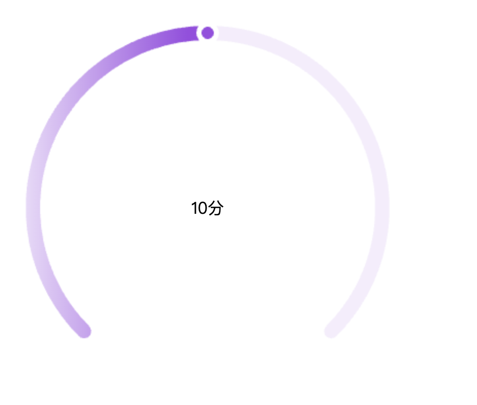
js:使用canvas画一个半圆
背景 需求需要画一个半圆,或者多半圆,其实一下子就能想到 canvas 中的圆弧,核心使用 context.arc context.arc(x,y,r,sAngle,eAngle,counterclockwise)接下来我们看看示例 例一 <!DOCTYPE html> <html lang"en"> &…...

1.框架介绍项目环境配置与项目启动!
目录 1.框架开发方向:2.项目启动与环境搭建 1.框架开发方向: 1.前后端分离项目 2.纯后端项目 3.移动端开发uni-app(ios、Android、H5、微信小程序) 4.内容管理系统2.项目启动与环境搭建 1.安装node.js 下载地址可以用nvm安装 便于运行前端项目https://juejin.cn/post/7094576…...

LeetCode算法题解:螺旋矩阵
LeetCode算法题解:螺旋矩阵 题目描述 给定一个 m x n 的矩阵,按照螺旋顺序返回矩阵中的所有元素。 解题思路 1. 初始化变量 我们首先定义四个边界变量来跟踪螺旋遍历的边界:top、bottom、left 和 right。 2. 螺旋遍历 开始从左到右遍历…...

【Java 设计模式】设计原则之开放封闭原则
文章目录 1. 定义2. 好处3. 应用4. 示例结语 在软件开发中,设计原则是创建灵活、可维护和可扩展软件的基础。 这些原则为我们提供了指导方针,帮助我们构建高质量、易理解的代码。 ✨单一职责原则(SRP) ✨开放/封闭原则(…...

数据分析求职-知识脑图
今天和大家聊聊数据分析求职常见面试题,这是这个系列的第一篇文章,但是我不想开始就直接罗列题目,因为这样的文章实在太多了,同学们的兴趣程度肯定一般。所以,我想先和大家聊聊在准备面试题时候通常遇到的困扰…...

SQL-修改数据
🎉欢迎您来到我的MySQL基础复习专栏 ☆* o(≧▽≦)o *☆哈喽~我是小小恶斯法克🍹 ✨博客主页:小小恶斯法克的博客 🎈该系列文章专栏:重拾MySQL 🍹文章作者技术和水平很有限,如果文中出现错误&am…...

Rockchip | FIQ-Debugger调试工具
FIQ-Debugger fiq debugger是集成到内核中的一种系统调试手段。 FIQ在arm架构中相当于nmi中断,fiq debugger把串口注册成fiq中断,在串口fiq中断服务程序中集成了一些系统调试命令。 一般情况下串口是普通的console模式,在串口工具下键盘输入…...

第二百六十三回 给geolocator插件提交问题
文章目录 1. 知识回顾2. 问题描述与解决2.1 问题描述2.2 问题解决 3. 心得与感受 1. 知识回顾 我们在前面章回中介绍过如何获取位置信息,主要介绍的是geolocator这个三方包,不过在最近使用时却发现了问题,尝试搜索解决,但是没有结…...

分组背包问题
题目来源:9. 分组背包问题 - AcWing题库 题目: 有 N 组物品和一个容量是 V 的背包。 每组物品有若干个,同一组内的物品最多只能选一个。 每件物品的体积是 vij,价值是 wij,其中 i 是组号,j 是组内编号。 …...

WinForm 中Label自动换行 解决方法
Label自动换行 1.单行完全显示:Label.AutoSize true; 2.换行显示:Label. AutoSize false;(Label框高度用户指定)。 3.多行显示 根据字数自动控制高度:Label.AutoSize true;Label.MaximumSize new Size(w,0); …...
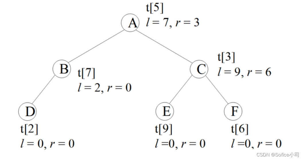
【蓝桥杯软件赛 零基础备赛20周】第7周——二叉树
文章目录 1 二叉树概念2 二叉树的存储和编码2.1 二叉树的存储方法2.2 二叉树存储的编码实现2.3 二叉树的极简存储方法 3 例题4 习题 前面介绍的数据结构数组、队列、栈,都是线性的,它们存储数据的方式是把相同类型的数据按顺序一个接一个串在一起。简单的…...

RestClient
什么是RestClient RestClient 是 Elasticsearch 官方提供的 Java 低级 REST 客户端,它允许HTTP与Elasticsearch 集群通信,而无需处理 JSON 序列化/反序列化等底层细节。它是 Elasticsearch Java API 客户端的基础。 RestClient 主要特点 轻量级ÿ…...

TDengine 快速体验(Docker 镜像方式)
简介 TDengine 可以通过安装包、Docker 镜像 及云服务快速体验 TDengine 的功能,本节首先介绍如何通过 Docker 快速体验 TDengine,然后介绍如何在 Docker 环境下体验 TDengine 的写入和查询功能。如果你不熟悉 Docker,请使用 安装包的方式快…...

Python:操作 Excel 折叠
💖亲爱的技术爱好者们,热烈欢迎来到 Kant2048 的博客!我是 Thomas Kant,很开心能在CSDN上与你们相遇~💖 本博客的精华专栏: 【自动化测试】 【测试经验】 【人工智能】 【Python】 Python 操作 Excel 系列 读取单元格数据按行写入设置行高和列宽自动调整行高和列宽水平…...

大语言模型如何处理长文本?常用文本分割技术详解
为什么需要文本分割? 引言:为什么需要文本分割?一、基础文本分割方法1. 按段落分割(Paragraph Splitting)2. 按句子分割(Sentence Splitting)二、高级文本分割策略3. 重叠分割(Sliding Window)4. 递归分割(Recursive Splitting)三、生产级工具推荐5. 使用LangChain的…...

智能分布式爬虫的数据处理流水线优化:基于深度强化学习的数据质量控制
在数字化浪潮席卷全球的今天,数据已成为企业和研究机构的核心资产。智能分布式爬虫作为高效的数据采集工具,在大规模数据获取中发挥着关键作用。然而,传统的数据处理流水线在面对复杂多变的网络环境和海量异构数据时,常出现数据质…...

【从零学习JVM|第三篇】类的生命周期(高频面试题)
前言: 在Java编程中,类的生命周期是指类从被加载到内存中开始,到被卸载出内存为止的整个过程。了解类的生命周期对于理解Java程序的运行机制以及性能优化非常重要。本文会深入探寻类的生命周期,让读者对此有深刻印象。 目录 …...

Windows安装Miniconda
一、下载 https://www.anaconda.com/download/success 二、安装 三、配置镜像源 Anaconda/Miniconda pip 配置清华镜像源_anaconda配置清华源-CSDN博客 四、常用操作命令 Anaconda/Miniconda 基本操作命令_miniconda创建环境命令-CSDN博客...
)
安卓基础(Java 和 Gradle 版本)
1. 设置项目的 JDK 版本 方法1:通过 Project Structure File → Project Structure... (或按 CtrlAltShiftS) 左侧选择 SDK Location 在 Gradle Settings 部分,设置 Gradle JDK 方法2:通过 Settings File → Settings... (或 CtrlAltS)…...

Oracle11g安装包
Oracle 11g安装包 适用于windows系统,64位 下载路径 oracle 11g 安装包...

【HarmonyOS 5】鸿蒙中Stage模型与FA模型详解
一、前言 在HarmonyOS 5的应用开发模型中,featureAbility是旧版FA模型(Feature Ability)的用法,Stage模型已采用全新的应用架构,推荐使用组件化的上下文获取方式,而非依赖featureAbility。 FA大概是API7之…...