数据分析(一) 理解数据
1. 描述性统计(summary)
对于一个新数据集,首先通过观察来熟悉它,可以打印数据相关信息来大致观察数据的常规特点,比如数据规模(行数列数)、数据类型、类别数量(变量数目、取值范围)、缺失值、异常值等等。然后通过描述性统计来了解数据的统计特性、属性间关联关系、属性与标签的关联关系等。
数据集一般是按照行列组织的,每行代表一个实例,每列代表一个属性。
import pandas as pd
import sys
import numpy as np
import pylab
import matplotlib.pyplot as plt
data = pd.read_csv(r"C:\work\PycharmProjects\machine_learning\filename.csv", index_col=0)
# summary
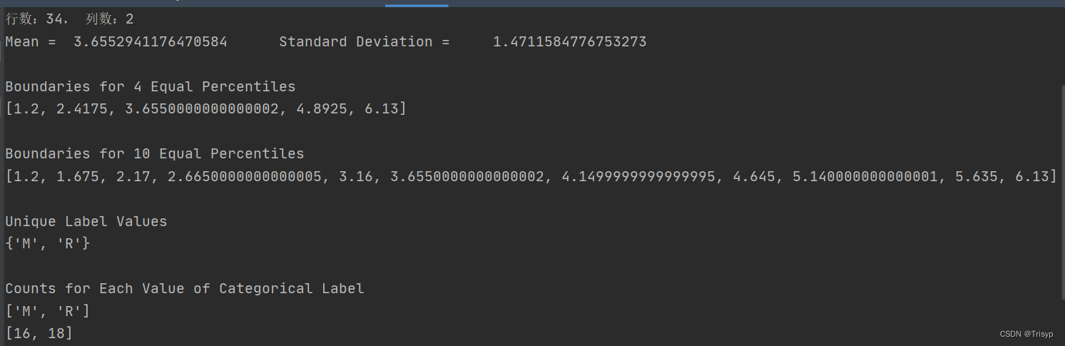
nrow, ncol = data.shape
print(f"行数:{nrow}, 列数:{ncol}")
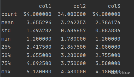
summary = data.describe()
print(summary)
# 箱线图
data_array = data.iloc[:, :3].values
pylab.boxplot(data_array)
plt.xlabel("Attribute Index")
plt.ylabel(("Quartile Ranges"))
pylab.show()
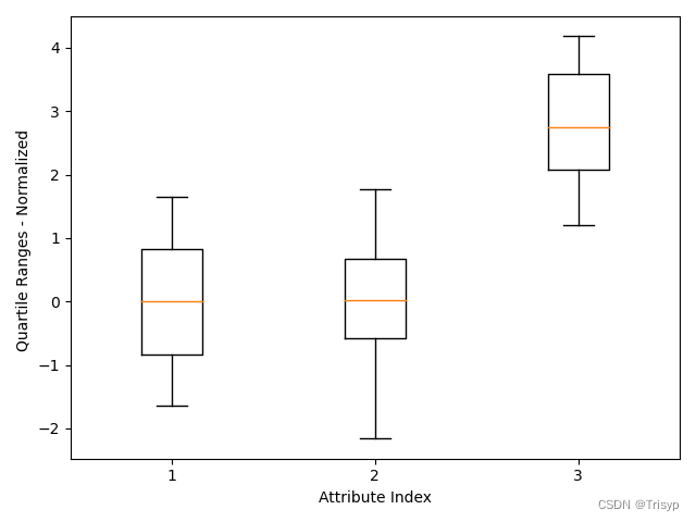
# 标准化后的箱线图
dataNormalized = data.iloc[:, :3]
for i in range(2):
mean = summary.iloc[1, i]
sd = summary.iloc[2, i]
dataNormalized.iloc[:, i:(i + 1)] = (dataNormalized.iloc[:, i:(i + 1)] - mean) / sd
array3 = dataNormalized.values
pylab.boxplot(array3)
plt.xlabel("Attribute Index")
plt.ylabel(("Quartile Ranges - Normalized "))
pylab.show()
colArray = np.array(list(data.iloc[:, 0]))
colMean = np.mean(colArray)
colsd = np.std(colArray)
sys.stdout.write("Mean = " + '\t' + str(colMean) + '\t\t' +
"Standard Deviation = " + '\t ' + str(colsd) + "\n")
# calculate quantile boundaries(四分位数边界)
ntiles = 4
percentBdry = []
for i in range(ntiles + 1):
percentBdry.append(np.percentile(colArray, i * (100) / ntiles))
sys.stdout.write("\nBoundaries for 4 Equal Percentiles \n")
print(percentBdry)
sys.stdout.write(" \n")
# run again with 10 equal intervals(十分位数边界)
ntiles = 10
percentBdry = []
for i in range(ntiles + 1):
percentBdry.append(np.percentile(colArray, i * (100) / ntiles))
sys.stdout.write("Boundaries for 10 Equal Percentiles \n")
print(percentBdry)
sys.stdout.write(" \n")
# The last column contains categorical variables(标签变量)
colData = list(data.iloc[:, 1])
unique = set(colData)
sys.stdout.write("Unique Label Values \n")
print(unique)
# count up the number of elements having each value
catDict = dict(zip(list(unique), range(len(unique))))
catCount = [0] * 2
for elt in colData:
catCount[catDict[elt]] += 1
sys.stdout.write("\nCounts for Each Value of Categorical Label \n")
print(list(unique))
print(catCount)
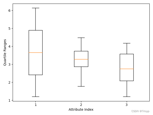
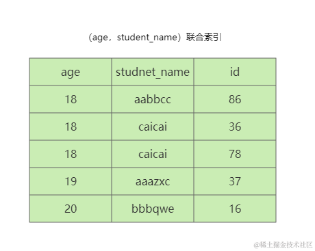
图中显示了一个小长方形,有一个红线穿过它。红线代表此列数据的中位数(第 50 百分位数),长方形的顶和底分别表示第 25 百分位数和第 75 百分位数(或者第一四分位数、第三四分位数)。在盒子的上方和下方有小的水平线,叫作盒须(whisker)。它们分别据盒子的上边和下边是四分位间距的 1.4 倍,四分位间距就是第 75 百分位数和第 25 百分位数之间的距离,也就是从盒子的顶边到盒子底边的距离。也就是说盒子上面的盒须到盒子顶边的距离是盒子高度的 1.4 倍。这个盒须的 1.4 倍距离是可以调整的(详见箱线图的相关文档)。在有些情况下,盒须要比 1.4 倍距离近,这说明数据的值并没有扩散到原定计算出来的盒须的位置。在这种情况下,盒须被放在最极端的点上。在另外一些情况下,数据扩散到远远超出计算出的盒须的位置(1.4 倍盒子高度的距离),这些点被认为是异常点。
2. 二阶统计信息(distribute,corr)
# 分位数图
import scipy.stats as stats
import pylab
stats.probplot(colArray, dist="norm", plot=pylab)
pylab.show()

如果此数据服从高斯分布,则画出来的点应该是接近一条直线。
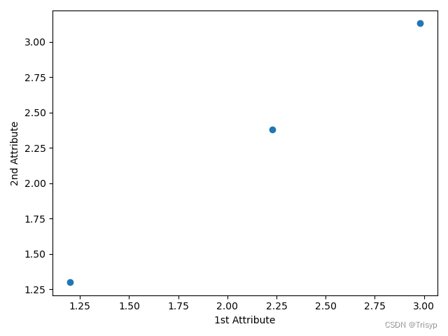
# 属性间关系散点图
import matplotlib.pyplot as plt
data_row1 = data.iloc[0, :3]
data_row2 = data.iloc[1, :3]
plt.scatter(data_row1, data_row2)
plt.xlabel("1st Attribute")
plt.ylabel(("2nd Attribute"))
plt.show()
# 属性和标签相关性散点图
from random import uniform
target = []
for i in range(len(colData)):
if colData[i] == 'R': # R用1代表, M用0代表
target.append(1)
else:
target.append(0)
plt.scatter(data_row1, target)
plt.xlabel("Attribute Value")
plt.ylabel("Target Value")
plt.show()
target = []
for i in range(len(colData)):
if colData[i] == 'R': # R用1代表, M用0代表
target.append(1+uniform(-0.1, 0.1))
else:
target.append(0+uniform(-0.1, 0.1))
plt.scatter(data_row1, target, alpha=0.5, s=120) # 透明度50%
plt.xlabel("Attribute Value")
plt.ylabel("Target Value")
plt.show()

第二个图绘制时取 alpha=0.5,这样这些点就是半透明的。那么在散点图中若多个点落在一个位置就会形成一个更黑的区域。

# 关系矩阵及其热图
corMat = pd.DataFrame(data.corr())
plt.pcolor(corMat)
plt.show()

属性之间如果完全相关(相关系数 =1)意味着数据可能有错误,如同样的数据录入两次。多个属性间的相关性很高(相关系数 >0.7),即多重共线性(multicollinearity),往往会导致预测结果不稳定。属性与标签的相关性则不同,如果属性和标签相关,则通常意味着两者之间具有可预测的关系
# 平行坐标图
minRings = summary.iloc[3, 2] # summary第3行为min
maxRings = summary.iloc[7, 2] # summary第7行为max
for i in range(nrow):
# plot rows of data as if they were series data
dataRow = data.iloc[i, :3]
labelColor = (data.iloc[i, 2] - minRings) / (maxRings - minRings)
dataRow.plot(color=plt.cm.RdYlBu(labelColor), alpha=0.5)
plt.xlabel("Attribute Index")
plt.ylabel(("Attribute Values"))
plt.show()
# 对数变换后平行坐标图
meanRings = summary.iloc[1, 2]
sdRings = summary.iloc[2, 2]
for i in range(nrow):
dataRow = data.iloc[i, :3]
normTarget = (data.iloc[i, 2] - meanRings) / sdRings
labelColor = 1.0 / (1.0 + np.exp(-normTarget))
dataRow.plot(color=plt.cm.RdYlBu(labelColor), alpha=0.5)
plt.xlabel("Attribute Index")
plt.ylabel(("Attribute Values"))
plt.show()
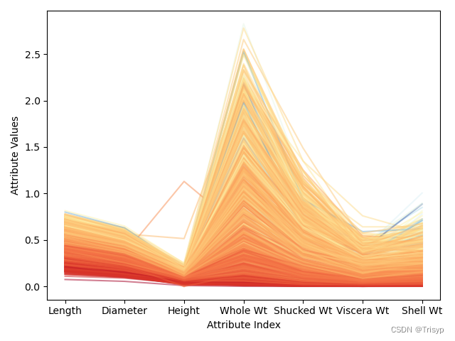
在属性值相近的地方,折线的颜色也比较接近,则会集中在一起。这些相关性都暗示可以构建相当准确的预测模型。相反,有些微弱的蓝色折线与深橘色的区域混合在一起,说明有些实例可能很难正确预测。
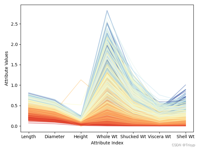
转换后可以更充分地利用颜色标尺中的各种颜色。注意到针对某些个属性,有些深蓝的线(对应年龄大的品种)混入了浅蓝线的区域,甚至是黄色、亮红的区域。这意味着,当该属性值较大时,仅仅这些属性不足以准确地预测出鲍鱼的年龄。好在其他属性可以很好地把深蓝线区分出来。这些观察都有助于分析预测错误的原因。
3. 完整代码(code)
import pandas as pd
import sys
import numpy as np
import pylab
import matplotlib.pyplot as pltdata = pd.read_csv(r"C:\work\PycharmProjects\machine_learning\filename.csv", index_col=0)nrow, ncol = data.shape
print(f"行数:{nrow}, 列数:{ncol}")
summary = data.describe()
print(summary)data_array = data.iloc[:, :3].values
pylab.boxplot(data_array)
plt.xlabel("Attribute Index")
plt.ylabel(("Quartile Ranges"))
pylab.show()dataNormalized = data.iloc[:, :3]
for i in range(2):mean = summary.iloc[1, i]sd = summary.iloc[2, i]dataNormalized.iloc[:, i:(i + 1)] = (dataNormalized.iloc[:, i:(i + 1)] - mean) / sdarray3 = dataNormalized.values
pylab.boxplot(array3)
plt.xlabel("Attribute Index")
plt.ylabel(("Quartile Ranges - Normalized "))
pylab.show()colArray = np.array(list(data.iloc[:, 0]))
colMean = np.mean(colArray)
colsd = np.std(colArray)
sys.stdout.write("Mean = " + '\t' + str(colMean) + '\t\t' +"Standard Deviation = " + '\t ' + str(colsd) + "\n")# calculate quantile boundaries(四分位数边界)
ntiles = 4
percentBdry = []
for i in range(ntiles + 1):percentBdry.append(np.percentile(colArray, i * (100) / ntiles))sys.stdout.write("\nBoundaries for 4 Equal Percentiles \n")
print(percentBdry)
sys.stdout.write(" \n")# run again with 10 equal intervals(十分位数边界)
ntiles = 10
percentBdry = []
for i in range(ntiles + 1):percentBdry.append(np.percentile(colArray, i * (100) / ntiles))
sys.stdout.write("Boundaries for 10 Equal Percentiles \n")
print(percentBdry)
sys.stdout.write(" \n")# The last column contains categorical variables(标签变量)
colData = list(data.iloc[:, 3])
unique = set(colData)
sys.stdout.write("Unique Label Values \n")
print(unique)# count up the number of elements having each value
catDict = dict(zip(list(unique), range(len(unique))))
catCount = [0] * 2
for elt in colData:catCount[catDict[elt]] += 1
sys.stdout.write("\nCounts for Each Value of Categorical Label \n")
print(list(unique))
print(catCount)# 分位数图
import scipy.stats as statsstats.probplot(colArray, dist="norm", plot=pylab)
pylab.show()# 属性间关系散点图
data_row1 = data.iloc[:, 0]
data_row2 = data.iloc[:, 1]
plt.scatter(data_row1, data_row2)
plt.xlabel("1st Attribute")
plt.ylabel(("2nd Attribute"))
plt.show()# 属性和标签相关性散点图
from random import uniformtarget = []
for i in range(len(colData)):if colData[i] == 'R':  # R用1代表, M用0代表target.append(1)else:target.append(0)
plt.scatter(data_row1, target)
plt.xlabel("Attribute Value")
plt.ylabel("Target Value")
plt.show()target = []
for i in range(len(colData)):if colData[i] == 'R':  # R用1代表, M用0代表target.append(1 + uniform(-0.1, 0.1))else:target.append(0 + uniform(-0.1, 0.1))
plt.scatter(data_row1, target, alpha=0.5, s=120)  # 透明度50%
plt.xlabel("Attribute Value")
plt.ylabel("Target Value")
plt.show()# 关系矩阵及其热图
corMat = pd.DataFrame(data.corr())
plt.pcolor(corMat)
plt.show()# 平行坐标图
minRings = summary.iloc[3, 2]  # summary第3行为min
maxRings = summary.iloc[7, 2]  # summary第7行为max
for i in range(nrow):# plot rows of data as if they were series datadataRow = data.iloc[i, :3]labelColor = (data.iloc[i, 2] - minRings) / (maxRings - minRings)dataRow.plot(color=plt.cm.RdYlBu(labelColor), alpha=0.5)
plt.xlabel("Attribute Index")
plt.ylabel(("Attribute Values"))
plt.show()meanRings = summary.iloc[1, 2]
sdRings = summary.iloc[2, 2]
for i in range(nrow):dataRow = data.iloc[i, :3]normTarget = (data.iloc[i, 2] - meanRings) / sdRingslabelColor = 1.0 / (1.0 + np.exp(-normTarget))dataRow.plot(color=plt.cm.RdYlBu(labelColor), alpha=0.5)
plt.xlabel("Attribute Index")
plt.ylabel(("Attribute Values"))
plt.show()
相关文章:
数据分析(一) 理解数据
1. 描述性统计(summary) 对于一个新数据集,首先通过观察来熟悉它,可以打印数据相关信息来大致观察数据的常规特点,比如数据规模(行数列数)、数据类型、类别数量(变量数目、取值范围…...

什么是 Flet?
什么是 Flet? Flet 是一个框架,允许使用您喜欢的语言构建交互式多用户 Web、桌面和移动应用程序,而无需前端开发经验。 您可以使用基于 Google 的 Flutter 的 Flet 控件为程序构建 UI。Flet 不只是“包装”Flutter 小部件,而是…...
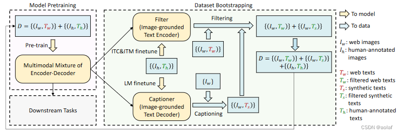
多模态(三)--- BLIP原理与源码解读
1 BLIP简介 BLIP: Bootstrapping Language-Image Pre-training for Unified Vision-Language Understanding and Generation 传统的Vision-Language Pre-training (VLP)任务大多是基于理解的任务或基于生成的任务,同时预训练数据多是从web获…...
掌握高性能SQL的34个秘诀多维度优化与全方位指南
掌握高性能SQL的34个秘诀🚀多维度优化与全方位指南 本篇文章从数据库表结构设计、索引、使用等多个维度总结出高性能SQL的34个秘诀,助你轻松掌握高性能SQL 表结构设计 字段类型越小越好 满足业务需求的同时字段类型越小越好 字段类型越小代表着记录占…...

美国纳斯达克大屏怎么投放:投放完成需要多长时间-大舍传媒Dashe Media
陕西大舍广告传媒有限公司(Shaanxi Dashe Advertising Media Co., Ltd),简称大舍传媒(Dashe Media),是纳斯达克在中国区的总代理(China General Agent)。与纳斯达克合作已经有八年的…...

【MySQL】多表关系的基本学习
🌈个人主页: Aileen_0v0 🔥热门专栏: 华为鸿蒙系统学习|计算机网络|数据结构与算法 💫个人格言:“没有罗马,那就自己创造罗马~” #mermaid-svg-3oES1ZdkKIklfKzq {font-family:"trebuchet ms",verdana,arial,sans-serif;font-siz…...
Springboot之接入gRPC
1、maven依赖 <properties><!-- grpc --><protobuf.version>3.5.1</protobuf.version><protobuf-plugin.version>0.6.1</protobuf-plugin.version><grpc.version>1.42.1</grpc.version><os-maven-plugin.version>1.6.0…...

2023年中国数据智能管理峰会(DAMS上海站2023):核心内容与学习收获(附大会核心PPT下载)
随着数字经济的飞速发展,数据已经渗透到现代社会的每一个角落,成为驱动企业创新、提升治理能力、促进经济发展的关键要素。在这样的背景下,2023年中国数据智能管理峰会(DAMS上海站2023)应运而生,汇聚了众多…...

DS:八大排序之堆排序、冒泡排序、快速排序
创作不易,友友们给个三连吧!! 一、堆排序 堆排序已经在博主关于堆的实现过程中详细的讲过了,大家可以直接去看,很详细,这边不介绍了 DS:二叉树的顺序结构及堆的实现-CSDN博客 直接上代码: …...

Sora:继ChatGPT之后,OpenAI的又一力作
关于Sora的报道,相信很多圈内朋友都已经看到了来自各大媒体铺天盖地的宣传了,这次,对于Sora的宣传,绝不比当初ChatGPT的宣传弱。自OpenAI发布了GPT4之后,就已经有很多视频生成模型了,不过这些模型要么生成的…...

阅读笔记(BMSB 2018)Video Stitching Based on Optical Flow
参考文献 Xie C, Zhang X, Yang H, et al. Video Stitching Based on Optical Flow[C]//2018 IEEE International Symposium on Broadband Multimedia Systems and Broadcasting (BMSB). IEEE, 2018: 1-5. 摘要 视频拼接在计算机视觉中仍然是一个具有挑战性的问题࿰…...

Ubuntu学习笔记-Ubuntu搭建禅道开源版及基本使用
文章目录 概述一、Ubuntu中安装1.1 复制下载安装包路径1.2 将安装包解压到ubuntu中1.3 启动服务1.4 设置开机自启动 二、禅道服务基本操作2.1 启动,停止,重启,查看服务状态2.2 开放端口2.3 访问和登录禅道 卜相机关 卜三命、相万生࿰…...
《苍穹外卖》知识梳理6-缓存商品,购物车功能
苍穹外卖实操笔记六—缓存商品,购物车功能 一.缓存菜品 可以使用redis进行缓存;另外,在实现缓存套餐时可以使用spring cache提高开发效率; 通过缓存数据,降低访问数据库的次数; 使用的缓存逻辑&#…...

[NSSCTF]-Web:[SWPUCTF 2021 新生赛]easy_sql解析
查看网页 有提示,参数是wllm,并且要我们输入点东西 所以,我们尝试以get方式传入 有回显,但似乎没啥用 从上图看应该是字符型漏洞,单引号字符注入 先查看字段数 /?wllm2order by 3-- 没回显 报错了,说明…...

vue3 codemirror yaml文件编辑器插件
需求:前端编写yaml配置文件 ,检查yaml语法 提供语法高亮 。 默认内容从后端接口获取 显示在前端 , 前端在codemirror 插件中修改文件内容 ,并提交修改 后端将提交的内容写入服务器配置文件中 。 codemirror 通过ref 后期编辑器…...

力扣经典题:环形链表的检测与返回
1.值得背的题 /*** Definition for singly-linked list.* struct ListNode {* int val;* struct ListNode *next;* };*/ struct ListNode *detectCycle(struct ListNode *head) {struct ListNode*fasthead;struct ListNode*slowhead;while(fast!NULL&&fast->…...
【web | CTF】BUUCTF [BJDCTF2020]Easy MD5
天命:好像也挺实用的题目,也是比较经典吧 天命:把php的MD5漏洞都玩了一遍 第一关:MD5绕过 先声明一下:这题的MD5是php,不是mysql的MD5,把我搞迷糊了 一进来题目啥也没有,那么就要看…...

spring boot Mybatis Plus分页
文章目录 Mybatis Plus自带分页和PageHelper有什么区别?Mybatis Plus整合PageHelper分页 springboot自定义拦截器获取分页参数spring boot下配置mybatis-plus分页插件单表分页查询自定义sql分页查询PageHelper 参考 Mybatis Plus自带分页和PageHelper有什么区别&…...
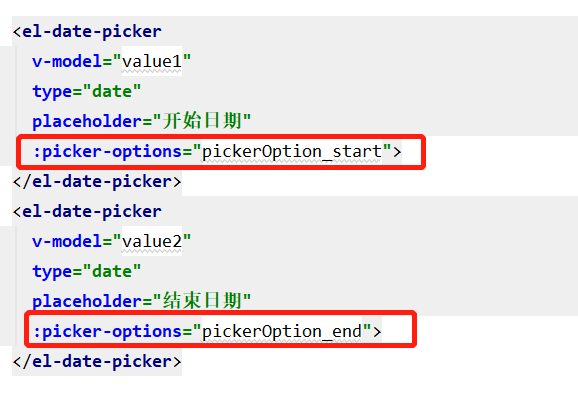
elementui 中 el-date-picker 控制选择当前年之前或者之后的年份
文章目录 需求分析 需求 对 el-date-picker控件做出判断控制 分析 给 el-date-picker 组件添加 picker-options 属性,并绑定对应数据 pickerOptions html <el-form-item label"雨量年份:" prop"date"><el-date-picker …...

GlusterFS:开源分布式文件系统的深度解析与应用场景实践
引言 在当今大数据时代背景下,企业对存储系统的容量、性能和可靠性提出了前所未有的挑战。GlusterFS作为一款开源的、高度可扩展的分布式文件系统,以其独特的无中心元数据设计和灵活的卷管理机制,在众多场景中脱颖而出,为解决大规…...
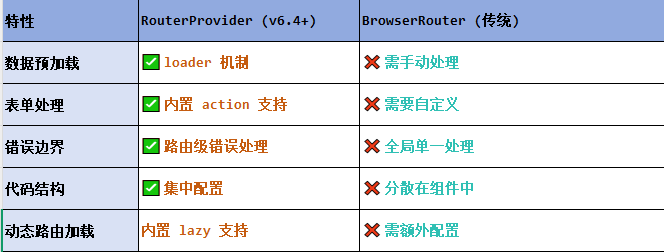
React第五十七节 Router中RouterProvider使用详解及注意事项
前言 在 React Router v6.4 中,RouterProvider 是一个核心组件,用于提供基于数据路由(data routers)的新型路由方案。 它替代了传统的 <BrowserRouter>,支持更强大的数据加载和操作功能(如 loader 和…...
Cesium相机控制)
三维GIS开发cesium智慧地铁教程(5)Cesium相机控制
一、环境搭建 <script src"../cesium1.99/Build/Cesium/Cesium.js"></script> <link rel"stylesheet" href"../cesium1.99/Build/Cesium/Widgets/widgets.css"> 关键配置点: 路径验证:确保相对路径.…...

Java如何权衡是使用无序的数组还是有序的数组
在 Java 中,选择有序数组还是无序数组取决于具体场景的性能需求与操作特点。以下是关键权衡因素及决策指南: ⚖️ 核心权衡维度 维度有序数组无序数组查询性能二分查找 O(log n) ✅线性扫描 O(n) ❌插入/删除需移位维护顺序 O(n) ❌直接操作尾部 O(1) ✅内存开销与无序数组相…...

【SpringBoot】100、SpringBoot中使用自定义注解+AOP实现参数自动解密
在实际项目中,用户注册、登录、修改密码等操作,都涉及到参数传输安全问题。所以我们需要在前端对账户、密码等敏感信息加密传输,在后端接收到数据后能自动解密。 1、引入依赖 <dependency><groupId>org.springframework.boot</groupId><artifactId...
SpringBoot+uniapp 的 Champion 俱乐部微信小程序设计与实现,论文初版实现
摘要 本论文旨在设计并实现基于 SpringBoot 和 uniapp 的 Champion 俱乐部微信小程序,以满足俱乐部线上活动推广、会员管理、社交互动等需求。通过 SpringBoot 搭建后端服务,提供稳定高效的数据处理与业务逻辑支持;利用 uniapp 实现跨平台前…...
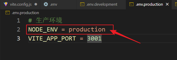
vue3+vite项目中使用.env文件环境变量方法
vue3vite项目中使用.env文件环境变量方法 .env文件作用命名规则常用的配置项示例使用方法注意事项在vite.config.js文件中读取环境变量方法 .env文件作用 .env 文件用于定义环境变量,这些变量可以在项目中通过 import.meta.env 进行访问。Vite 会自动加载这些环境变…...
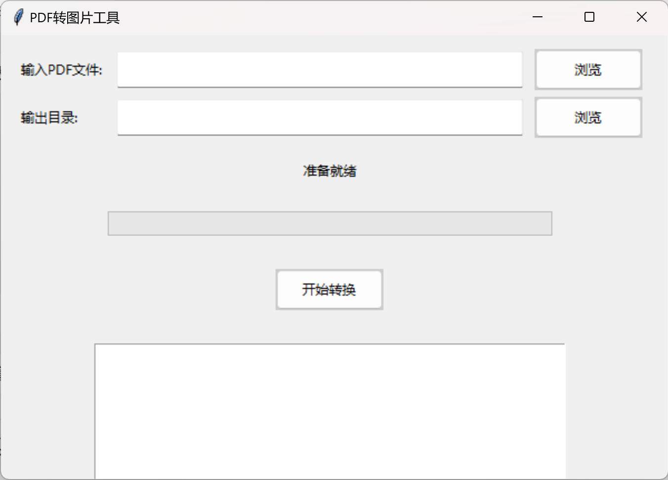
免费PDF转图片工具
免费PDF转图片工具 一款简单易用的PDF转图片工具,可以将PDF文件快速转换为高质量PNG图片。无需安装复杂的软件,也不需要在线上传文件,保护您的隐私。 工具截图 主要特点 🚀 快速转换:本地转换,无需等待上…...
深度学习水论文:mamba+图像增强
🧀当前视觉领域对高效长序列建模需求激增,对Mamba图像增强这方向的研究自然也逐渐火热。原因在于其高效长程建模,以及动态计算优势,在图像质量提升和细节恢复方面有难以替代的作用。 🧀因此短时间内,就有不…...
Python 实现 Web 静态服务器(HTTP 协议)
目录 一、在本地启动 HTTP 服务器1. Windows 下安装 node.js1)下载安装包2)配置环境变量3)安装镜像4)node.js 的常用命令 2. 安装 http-server 服务3. 使用 http-server 开启服务1)使用 http-server2)详解 …...
)
LLaMA-Factory 微调 Qwen2-VL 进行人脸情感识别(二)
在上一篇文章中,我们详细介绍了如何使用LLaMA-Factory框架对Qwen2-VL大模型进行微调,以实现人脸情感识别的功能。本篇文章将聚焦于微调完成后,如何调用这个模型进行人脸情感识别的具体代码实现,包括详细的步骤和注释。 模型调用步骤 环境准备:确保安装了必要的Python库。…...