Opencv Python图像处理笔记二:图像变换、卷积、形态学变换
文章目录
- 前言
- 一、几何变换
- 1.1 缩放
- 1.2 平移
- 1.3 旋转
- 1.4 翻转
- 1.5 仿射
- 1.6 透视
- 二、低通滤波
- 2.1 均值滤波
- 2.2 高斯滤波
- 2.3 中值滤波
- 2.4 双边滤波
- 2.5 自定义滤波
- 三、高通滤波
- 3.1 Sobel
- 3.2 Scharr
- 3.3 Laplacian
- 3.4 Canny
- 四、图像金字塔
- 4.1 高斯金字塔
- 4.2 拉普拉斯金字塔
- 五、形态学
- 5.1 腐蚀
- 5.2 膨胀
- 5.3 运算
- 六、直方图
- 6.1 计算
- 6.2 均衡
- 6.3 反向投影
- 七、轮廓
- 7.1 查找显示
- 7.2 常用特征
- 参考
前言
图像处理是计算机视觉领域中的核心技术之一,它涉及到对图像进行各种变换、滤波、金字塔构建、形态学操作等一系列处理。在本篇博文中,我们将深入探讨使用OpenCV和Python进行图像处理的各种技术和方法。从几何变换到滤波、金字塔构建再到形态学操作,我们将逐步介绍并实践这些重要的图像处理技术,帮助读者更好地理解和应用于实际项目中。
一、几何变换
1.1 缩放
import cv2 as cv
import numpy as np
from matplotlib import pyplot as pltdef generateCanvas(img, img2):canvas = np.zeros((max(img.shape[0], img2.shape[0]),img.shape[1] + img2.shape[1], 3), dtype=np.uint8)# 将图像1和图像2放置在画布上canvas[:img.shape[0], :img.shape[1]] = imgcanvas[:img2.shape[0],img.shape[1]:] = img2return canvasdef main():img = cv.imread('sudoku.png')assert img is not None, "file could not be read, check with os.path.exists()"# dsize:输出图像的大小。如果这个参数不为None,那么就代表将原图像缩放到这个Size(width,height)指定的大小;#        如果这个参数为0,那么原图像缩放之后的大小就要通过下面的公式来计算:#               dsize = Size(round(fx*src.cols), round(fy*src.rows))#       其中,fx和fy就是下面要说的两个参数,是图像width方向和height方向的缩放比例。#  fx:width方向的缩放比例,如果它是0,那么它就会按照(double)dsize.width/src.cols来计算;#  fy:height方向的缩放比例,如果它是0,那么它就会按照(double)dsize.height/src.rows来计算;# interpolation:这个是指定插值的方式,图像缩放之后,肯定像素要进行重新计算的,就靠这个参数来指定重新计算像素的方式,有以下几种:#     INTER_NEAREST              - 最近邻插值#     INTER_LINEAR               - 双线性插值,如果最后一个参数你不指定,默认使用这种方法#     INTER_AREA                 - 使用像素区域关系进行重采样#     INTER_CUBIC                - 4x4像素邻域内 的双立方插值#     INTER_LANCZOS4             - 8x8像素邻域内的Lanczos插值fx = 0.6fy = 0.6img_half_nearest = cv.resize(img, dsize=None, fx=fx, fy=fy, interpolation=cv.INTER_NEAREST)img_half_linear = cv.resize(img, dsize=None, fx=fx, fy=fy, interpolation=cv.INTER_LINEAR)img_half_area = cv.resize(img, dsize=None, fx=fx,fy=fy, interpolation=cv.INTER_AREA)img_half_cubic = cv.resize(img, dsize=None, fx=fx, fy=fy, interpolation=cv.INTER_CUBIC)img_half_lanczos4 = cv.resize(img, dsize=None, fx=fx, fy=fy, interpolation=cv.INTER_LANCZOS4)titles = ['nearest', 'linear', 'area', 'cubic', 'Lanczos']images = [img_half_nearest, img_half_linear,img_half_area, img_half_cubic, img_half_lanczos4]# canvas = generateCanvas(img, img_half_linear)# cv.imshow('test', canvas)for i in range(len(images)):show = cv.cvtColor(generateCanvas(img, images[i]), cv.COLOR_BGR2RGB)plt.subplot(2, 3, i+1), plt.imshow(show)plt.title(titles[i])plt.xticks([]), plt.yticks([])plt.show()cv.waitKey(0)cv.destroyAllWindows()if __name__ == '__main__':main()

1.2 平移
import cv2 as cv
import numpy as np
from matplotlib import pyplot as pltdef main():img = cv.imread('lena.png')assert img is not None, "file could not be read, check with os.path.exists()"rows, cols, _ = img.shapeM = np.float32([[1, 0, 100], [0, 1, 50]])# M: 2 * 3 矩阵# 根据下面的公式,想实现平移,可以通过构造M=[[1, 0, x], [0, 1, y]],实现向右平移x,向下平移y# dst(x, y) = (M[0,0] * x  + M[0, 1] * y + M[0, 2], M[1, 0] * x + M[1, 1] * y + M[1, 2])img_right_down = cv.warpAffine(img, M, (cols, rows))M = np.float32([[1, 0, -100], [0, 1, -50]])img_left_up = cv.warpAffine(img, M, (cols, rows))titles = ['origin', 'right down', 'left up']images = [img, img_right_down, img_left_up]for i in range(len(images)):show = cv.cvtColor(images[i], cv.COLOR_BGR2RGB)plt.subplot(1, 3, i+1), plt.imshow(show)plt.title(titles[i])plt.xticks([]), plt.yticks([])plt.show()cv.waitKey(0)cv.destroyAllWindows()if __name__ == '__main__':main()

1.3 旋转
import cv2 as cv
import numpy as np
from matplotlib import pyplot as pltdef main():img = cv.imread('lena.png')assert img is not None, "file could not be read, check with os.path.exists()"rows, cols, _ = img.shapeM = cv.getRotationMatrix2D(center=(rows / 2, cols / 2), angle=-30, scale=1)img_rotete_minus_30 = cv.warpAffine(img, M, (cols, rows))M = cv.getRotationMatrix2D(center=(rows / 2, cols / 2), angle=30, scale=1)img_rotete_30 = cv.warpAffine(img, M, (cols, rows))titles = ['origin', 'rotate -30 degree', 'rotate 30 degree']images = [img, img_rotete_minus_30, img_rotete_30]for i in range(len(images)):show = cv.cvtColor(images[i], cv.COLOR_BGR2RGB)plt.subplot(1, 3, i+1), plt.imshow(show)plt.title(titles[i])plt.xticks([]), plt.yticks([])plt.show()cv.waitKey(0)cv.destroyAllWindows()if __name__ == '__main__':main()

1.4 翻转
import cv2 as cv
import numpy as np
from matplotlib import pyplot as pltdef main():img = cv.imread('lena.png')assert img is not None, "file could not be read, check with os.path.exists()"# 竖直翻转img_vertical = cv.flip(img, flipCode=1)# 水平翻转img_horizontal = cv.flip(img, flipCode=0)# 两者img_both = cv.flip(img, flipCode=-1)title = ['Origin', 'flipCode=1,Vertical','flipCode=0,Horizontal', 'flipCode=-1,Both']# 对应的图像imgs = [img, img_vertical, img_horizontal, img_both]for i in range(len(imgs)):plt.subplot(2, 2, i + 1)plt.imshow(cv.cvtColor(imgs[i], cv.COLOR_BGR2RGB))plt.title(title[i])plt.axis('off')plt.show()cv.waitKey(0)cv.destroyAllWindows()if __name__ == '__main__':main()

1.5 仿射
import cv2 as cv
import numpy as np
from matplotlib import pyplot as pltdef main():img = cv.imread('lena.png')assert img is not None, "file could not be read, check with os.path.exists()"rows, cols, _ = img.shape# pts1 表示变换前三个点位置# pts2 表示变换后三个点位置pts1 = np.float32([[270, 270], [330, 270], [310, 320]])pts2 = np.float32([[100, 100], [150, 50], [150, 100]])M = cv.getAffineTransform(pts1, pts2)img_result = cv.warpAffine(img, M, (cols, rows))for p in pts1:cv.circle(img, center=(int(p[0]), int(p[1])), radius=3,color=(0, 0, 255), thickness=cv.FILLED)for p in pts2:cv.circle(img_result, center=(int(p[0]), int(p[1])), radius=3,color=(0, 255, 0), thickness=cv.FILLED)title = ['Origin', 'Affine']# 对应的图像imgs = [img, img_result]for i in range(len(imgs)):plt.subplot(1, len(imgs), i + 1)plt.imshow(cv.cvtColor(imgs[i], cv.COLOR_BGR2RGB))plt.title(title[i])plt.axis('off')plt.show()cv.waitKey(0)cv.destroyAllWindows()if __name__ == '__main__':main()

1.6 透视
import cv2 as cv
import numpy as np
from matplotlib import pyplot as pltdef main():img = cv.imread('lena.png')assert img is not None, "file could not be read, check with os.path.exists()"rows, cols, _ = img.shape# 将图像投影到一个新的视平面,需要四个点, 在这4个点中,有3个点不应共线# 平面的4个点顺序为 左上 右上 左下 右下pts1 = np.float32([[270, 270], [330, 270], [270, 350], [320, 350]])pts2 = np.float32([[0, 0], [512, 0], [0, 512], [512, 512]])M = cv.getPerspectiveTransform(pts1, pts2)img_result = cv.warpPerspective(img, M, (cols, rows))for p in pts1:cv.circle(img, center=(int(p[0]), int(p[1])), radius=3,color=(0, 0, 255), thickness=cv.FILLED)for p in pts2:cv.circle(img_result, center=(int(p[0]), int(p[1])), radius=3,color=(0, 255, 0), thickness=cv.FILLED)title = ['Origin', 'Perspective',]# 对应的图像imgs = [img, img_result]for i in range(len(imgs)):plt.subplot(1, len(imgs), i + 1)plt.imshow(cv.cvtColor(imgs[i], cv.COLOR_BGR2RGB))plt.title(title[i])plt.axis('off')plt.show()cv.waitKey(0)cv.destroyAllWindows()if __name__ == '__main__':main()

二、低通滤波
与一维信号一样,图像也可以用各种低通滤波器(low-pass filters,LPF)、高通滤波器(high-pass filters,HPF)等进行过滤
- LPF 用于降低某些像素强度,可以用于平滑图像,保留图像中的低频成分,过滤高频成分,帮助去除噪点,模糊图像等
- HPF 用于增强某些像素强度,可以用于帮助寻找图像中的边缘
2.1 均值滤波
import cv2 as cv
import numpy as np
from matplotlib import pyplot as pltdef main():img = cv.imread('lenaNoise.png')assert img is not None, "file could not be read, check with os.path.exists()"# 均值滤波: 简单的平均卷积操作result = cv.blur(img, ksize=(5, 5))# 显示图像titles = ['origin image', 'blur image']images = [img, result]for i in range(2):plt.subplot(1, 2, i+1), plt.imshow(cv.cvtColor(images[i], cv.COLOR_BGR2RGB))plt.title(titles[i])plt.axis('off')plt.tight_layout()plt.show()cv.waitKey(0)cv.destroyAllWindows()if __name__ == '__main__':main()

2.2 高斯滤波
import cv2 as cv
import numpy as np
from matplotlib import pyplot as pltdef main():img = cv.imread('lenaNoise.png')assert img is not None, "file could not be read, check with os.path.exists()"# 高斯滤波:# ksize: 高斯核大小,可以是0或正奇数,当为0从sigma计算result_0 = cv.GaussianBlur(img, ksize=(5, 5), sigmaX=0)# 显示图像titles = ['origin image', 'gaussian blur']images = [img, result_0]for i in range(len(images)):plt.subplot(1, len(images), i+1), plt.imshow(cv.cvtColor(images[i], cv.COLOR_BGR2RGB))plt.title(titles[i])plt.axis('off')plt.tight_layout()plt.show()cv.waitKey(0)cv.destroyAllWindows()if __name__ == '__main__':main()

2.3 中值滤波
import cv2 as cv
import numpy as np
from matplotlib import pyplot as pltdef main():img = cv.imread('lenaNoise.png')assert img is not None, "file could not be read, check with os.path.exists()"# 中值滤波:result_0 = cv.medianBlur(img, ksize=3)result_1 = cv.medianBlur(img, ksize=5)result_2 = cv.medianBlur(img, ksize=7)# 显示图像titles = ['origin image', 'ksize=3', 'ksize=5', 'ksize=7']images = [img, result_0, result_1, result_2]for i in range(len(images)):plt.subplot(2, 2, i+1), plt.imshow(cv.cvtColor(images[i], cv.COLOR_BGR2RGB))plt.title(titles[i])plt.axis('off')plt.show()cv.waitKey(0)cv.destroyAllWindows()if __name__ == '__main__':main()
2.4 双边滤波
import cv2 as cv
import numpy as np
from matplotlib import pyplot as pltdef main():img = cv.imread('lenaNoise.png')assert img is not None, "file could not be read, check with os.path.exists()"# 双边滤波: 在计算像素值的同时会考虑距离和色差信息,从而可在消除噪声得同时保护边缘信息,可用于美颜# d 每个像素邻域的直径,当<=0时,从sigmaSpace计算     注意:当 d > 5 非常慢,所以建议使用=5作为实时应用,或者使用=9作为需要重噪声过滤的离线应用# sigmaColor 颜色标准方差,一般尽可能大,较大的值表示在颜色相近的区域内像素将会被更多地保留# sigmaSpace 坐标空间标准方差(像素单位),一般尽可能小,较小的值表示在距离中心像素较远的像素的权重较小result_0 = cv.bilateralFilter(img, d=0, sigmaColor=100, sigmaSpace=15)result_1 = cv.bilateralFilter(img, d=0, sigmaColor=50, sigmaSpace=15)# 显示图像titles = ['origin image', 'color=100 space=5', 'color=50 space=5']images = [img, result_0, result_1]for i in range(len(images)):plt.subplot(1, len(images), i+1), plt.imshow(cv.cvtColor(images[i], cv.COLOR_BGR2RGB))plt.title(titles[i])plt.axis('off')plt.show()cv.waitKey(0)cv.destroyAllWindows()if __name__ == '__main__':main()

2.5 自定义滤波
import cv2 as cv
import numpy as np
from matplotlib import pyplot as pltdef main():img = cv.imread('lenaNoise.png')assert img is not None, "file could not be read, check with os.path.exists()"# 自定义滤波,对图像进行卷积运算:# 先定义卷积核,再参与计算,ddepth=-1表示和源图像深度一致# 此外还有个参数anchor,默认值为(-1,-1)表示锚点位于内核中心kernel = np.ones((5, 5), np.float32)/25result = cv.filter2D(img, ddepth=-1, kernel=kernel)# 显示图像titles = ['origin image', 'filter2d filter',]images = [img, result]for i in range(len(images)):plt.subplot(1, len(images), i+1), plt.imshow(cv.cvtColor(images[i], cv.COLOR_BGR2RGB))plt.title(titles[i])plt.axis('off')plt.show()cv.waitKey(0)cv.destroyAllWindows()if __name__ == '__main__':main()

三、高通滤波
3.1 Sobel
import cv2 as cv
import numpy as np
from matplotlib import pyplot as pltdef sobel(img):# Sobel 使用Sobel算子计算一阶、二阶、三阶或三者混合 图像导数梯度# ddepth 输出图像的深度,计算图像的梯度会有浮点数,负数,所以后面会取绝对值# dx,dy  X和Y方向的梯度# ksize  参与图像卷积操作的核,大小可以是1、3、5或7,用于不同精度的边缘检测grad_x = cv.Sobel(img, ddepth=cv.CV_64F, dx=1, dy=0, ksize=3)abs_grad_x = cv.convertScaleAbs(grad_x)grad_y = cv.Sobel(img, ddepth=cv.CV_64F, dx=0, dy=1, ksize=3)abs_grad_y = cv.convertScaleAbs(grad_y)# 分别计算x和y,再求和sobel = cv.addWeighted(abs_grad_x, 0.5, abs_grad_y, 0.5, 0)return abs_grad_x, abs_grad_y, sobeldef main():img = cv.imread('res2.jpg')img_lena = cv.imread('lena.png', cv.IMREAD_GRAYSCALE)assert img is not None and img_lena is not None, "file could not be read, check with os.path.exists()"# 显示图像titles = ['origin ', 'sobel_x', 'sobel_y', 'sobel_x+sobel_y', 'lena ','lena_sobel_x', 'lena_sobel_y', 'lena_sobel_x+lena_sobel_y']images = [img, *sobel(img), img_lena, *sobel(img_lena)]for i in range(len(images)):plt.subplot(2, 4, i+1)plt.imshow(cv.cvtColor(images[i], cv.COLOR_BGR2RGB))plt.title(titles[i])plt.axis('off')plt.show()cv.waitKey(0)cv.destroyAllWindows()if __name__ == '__main__':main()

3.2 Scharr
import cv2 as cv
import numpy as np
from matplotlib import pyplot as plt
plt.rcParams['font.sans-serif'] = ['SimHei']def main():img = cv.imread('lena.png', cv.IMREAD_GRAYSCALE)assert img is not None, "file could not be read, check with os.path.exists()"scharrx = cv.Scharr(img, ddepth=cv.CV_64F, dx=1, dy=0)scharrxAbs = cv.convertScaleAbs(scharrx)scharry = cv.Scharr(img, ddepth=cv.CV_64F, dx=0, dy=1)scharryAbs = cv.convertScaleAbs(scharry)# 分别计算x和y,再求和scharrxy = cv.addWeighted(scharrxAbs, 0.5, scharryAbs, 0.5, 0)# 显示图像titles = ['origin ', 'scharrx', 'scharry', 'scharrx + scharry']images = [img, scharrxAbs, scharryAbs, scharrxy]for i in range(len(images)):plt.subplot(2, 2, i+1)plt.imshow(cv.cvtColor(images[i], cv.COLOR_BGR2RGB))plt.title(titles[i])plt.axis('off')plt.tight_layout()plt.show()cv.waitKey(0)cv.destroyAllWindows()if __name__ == '__main__':main()

3.3 Laplacian
import cv2 as cv
import numpy as np
from matplotlib import pyplot as plt
plt.rcParams['font.sans-serif'] = ['SimHei']def main():img = cv.imread('lena.png', cv.IMREAD_GRAYSCALE)assert img is not None, "file could not be read, check with os.path.exists()"result = cv.Laplacian(img, cv.CV_16S, ksize=3)resultAbs = cv.convertScaleAbs(result)# 显示图像titles = ['origin ', 'Laplacian']images = [img, resultAbs]for i in range(len(images)):plt.subplot(1, 2, i+1)plt.imshow(cv.cvtColor(images[i], cv.COLOR_BGR2RGB))plt.title(titles[i])plt.axis('off')plt.show()cv.waitKey(0)cv.destroyAllWindows()if __name__ == '__main__':main()

3.4 Canny
import cv2 as cv
import numpy as np
from matplotlib import pyplot as plt
# plt.rcParams['font.sans-serif'] = ['SimHei']def main():img = cv.imread('lena.png')assert img is not None, "file could not be read, check with os.path.exists()"# canny 是一个多步算法,先用5*5核高斯滤波过滤噪声,然后用Sobel算法查找图像梯度,最后去除任何可能不构成边缘的、不需要的像素# threshold1 较小值 低于这个值的肯定不是边# threshold2 较大值 高于这个值的肯定是边# 位于两者之间的需要进行连通性判断img_gray = cv.cvtColor(img, cv.COLOR_BGR2GRAY)img_result_1 = cv.Canny(img_gray, threshold1=100, threshold2=200)img_result_2 = cv.Canny(img_gray, threshold1=50, threshold2=240)# 显示图像titles = ['origin ', 'gray', 'canny 100,200', 'canny 50,240']images = [img, img_gray, img_result_1, img_result_2]for i in range(len(images)):plt.subplot(2, 2, i+1)plt.imshow(cv.cvtColor(images[i], cv.COLOR_BGR2RGB))plt.title(titles[i])plt.axis('off')plt.tight_layout()plt.show()cv.waitKey(0)cv.destroyAllWindows()if __name__ == '__main__':main()

四、图像金字塔
通常,我们通常处理恒定大小的图像。但在某些情况下,我们需要处理不同分辨率的(相同的)图像。例如,当在图像中搜索某个东西时,比如人脸,我们不确定物体将在该图像中出现在什么大小。在这种情况下,我们将需要创建一组具有不同分辨率的相同图像,并在所有这些图像中搜索对象。这些不同分辨率的图像集被称为图像金字塔(因为当它们被保存在一个堆栈中,顶部是最高分辨率的图像时,它看起来就像一个金字塔)。
金字塔的一个应用是图像混合。
4.1 高斯金字塔
import cv2 as cv
import numpy as np
from matplotlib import pyplot as plt
plt.rcParams['font.sans-serif'] = ['SimHei']def main():img = cv.imread('lena.png')assert img is not None, "file could not be read, check with os.path.exists()"# 模糊图像向下采样img_down = cv.pyrDown(img)img_down_down = cv.pyrDown(img_down)img_down_down_down = cv.pyrDown(img_down_down)# 显示图像titles = ['origin ', '向下采样1', '向下采样2', '向下采样3']images = [img, img_down, img_down_down, img_down_down_down]for i in range(len(images)):plt.subplot(2, 2, i+1)plt.imshow(cv.cvtColor(images[i], cv.COLOR_BGR2RGB))plt.title(titles[i])plt.axis('off')plt.tight_layout()plt.show()cv.waitKey(0)cv.destroyAllWindows()if __name__ == '__main__':main()

4.2 拉普拉斯金字塔
拉普拉斯金字塔是由高斯金字塔形成的。拉普拉斯金字塔图像像边缘图像,它的大多数元素都是零,常被用于图像压缩。拉普拉斯金字塔的水平是由高斯金字塔的水平与高斯金字塔的扩展水平的差异形成的
import cv2 as cv
import numpy as np
from matplotlib import pyplot as plt
# plt.rcParams['font.sans-serif'] = ['SimHei']def main():img = cv.imread('lena.png')assert img is not None, "file could not be read, check with os.path.exists()"# pyrDown和pyrUp并不是可逆的img_down = cv.pyrDown(img)img_down_up = cv.pyrUp(img_down)img_laplacian = img - img_down_up# 显示图像titles = ['origin ', 'img_laplacian']images = [img, img_laplacian]for i in range(len(images)):plt.subplot(1, 2, i+1)plt.imshow(cv.cvtColor(images[i], cv.COLOR_BGR2RGB))plt.title(titles[i])plt.axis('off')plt.show()cv.waitKey(0)cv.destroyAllWindows()if __name__ == '__main__':main()

五、形态学
5.1 腐蚀
import cv2 as cv
import numpy as np
from matplotlib import pyplot as plt
# plt.rcParams['font.sans-serif'] = ['SimHei']def main():img = cv.imread('j.png')assert img is not None, "file could not be read, check with os.path.exists()"kernel3 = np.ones((3, 3), np.uint8)img_erode_3 = cv.erode(img, kernel3, iterations=1)kernel5 = np.ones((5, 5), np.uint8)img_erode_5 = cv.erode(img, kernel5, iterations=1)cross = cv.getStructuringElement(cv.MORPH_CROSS, (5, 5))img_erode_by_cross = cv.erode(img, cross)ellipse = cv.getStructuringElement(cv.MORPH_ELLIPSE, (5, 5))img_erode_by_ellipse = cv.erode(img, ellipse)# 显示图像titles = ['origin ', 'erode_3', 'erode_5', 'cross', 'ellipse']images = [img, img_erode_3, img_erode_5,img_erode_by_cross, img_erode_by_ellipse]for i in range(len(images)):plt.subplot(2, 3, i+1)plt.imshow(cv.cvtColor(images[i], cv.COLOR_BGR2RGB))plt.title(titles[i])plt.axis('off')plt.tight_layout()plt.show()cv.waitKey(0)cv.destroyAllWindows()if __name__ == '__main__':main()

5.2 膨胀
import cv2 as cv
import numpy as np
from matplotlib import pyplot as plt
# plt.rcParams['font.sans-serif'] = ['SimHei']def main():img = cv.imread('j.png')assert img is not None, "file could not be read, check with os.path.exists()"kernel3 = np.ones((3, 3), np.uint8)img_dilate_3 = cv.dilate(img, kernel3, iterations=1)kernel5 = np.ones((5, 5), np.uint8)img_dilate_5 = cv.dilate(img, kernel5, iterations=1)cross = cv.getStructuringElement(cv.MORPH_CROSS, (5, 5))img_dilate_by_cross = cv.dilate(img, cross)ellipse = cv.getStructuringElement(cv.MORPH_ELLIPSE, (5, 5))img_dilate_by_ellipse = cv.dilate(img, ellipse)# 显示图像titles = ['origin ', 'dilate_3', 'dilate_5', 'cross', 'ellipse']images = [img, img_dilate_3, img_dilate_5,img_dilate_by_cross, img_dilate_by_ellipse]for i in range(len(images)):plt.subplot(2, 3, i+1)plt.imshow(cv.cvtColor(images[i], cv.COLOR_BGR2RGB))plt.title(titles[i])plt.axis('off')plt.tight_layout()plt.show()cv.waitKey(0)cv.destroyAllWindows()if __name__ == '__main__':main()

5.3 运算
import cv2 as cv
import numpy as np
from matplotlib import pyplot as plt
# plt.rcParams['font.sans-serif'] = ['SimHei']def main():img = cv.imread('j.png')assert img is not None, "file could not be read, check with os.path.exists()"# 形态学通常用于二值化图像# 开操作:先腐蚀后膨胀# 闭操作:先膨胀后腐蚀# 形态学梯度:膨胀减去腐蚀。# 顶帽:原图像与开操作图像之间的差值图像。# 黑帽:闭操作图像与原图像之间的差值图像。kernel = np.ones((3, 3), np.uint8)img_opening = cv.morphologyEx(img, cv.MORPH_OPEN, kernel)img_closing = cv.morphologyEx(img, cv.MORPH_CLOSE, kernel)img_gradient = cv.morphologyEx(img, cv.MORPH_GRADIENT, kernel)img_tophat = cv.morphologyEx(img, cv.MORPH_TOPHAT, kernel)img_blackhat = cv.morphologyEx(img, cv.MORPH_BLACKHAT, kernel)# 显示图像titles = ['origin ', 'open', 'close', 'gradient', 'tophat', 'blackhat']images = [img, img_opening, img_closing,img_gradient, img_tophat, img_blackhat]for i in range(len(images)):plt.subplot(2, 3, i+1)plt.imshow(cv.cvtColor(images[i], cv.COLOR_BGR2RGB))plt.title(titles[i])plt.axis('off')plt.tight_layout()plt.show()cv.waitKey(0)cv.destroyAllWindows()if __name__ == '__main__':main()

六、直方图
6.1 计算
import cv2 as cv
import numpy as np
from matplotlib import pyplot as plt
# plt.rcParams['font.sans-serif'] = ['SimHei']def main():img = cv.imread('lena.png')assert img is not None, "file could not be read, check with os.path.exists()"img_gray = cv.cvtColor(img, cv.COLOR_BGR2GRAY)img_hist = cv.calcHist([img], [0], None, [256], [0, 256])# 显示图像titles = ['gray', 'origin']images = [img_gray, img]for i in range(len(images)):plt.subplot(2, 2, i+1)plt.imshow(cv.cvtColor(images[i], cv.COLOR_BGR2RGB))plt.title(titles[i])plt.axis('off')plt.subplot(2, 2, 3)plt.plot(img_hist)plt.title('histogram')plt.xlim([0, 256])color = ('b', 'g', 'r')plt.subplot(2, 2, 4)for i, col in enumerate(color):histr = cv.calcHist([img], [i], None, [256], [0, 256])plt.plot(histr, color=col)plt.xlim([0, 256])plt.title('color histogram')plt.tight_layout()plt.show()cv.waitKey(0)cv.destroyAllWindows()if __name__ == '__main__':main()

6.2 均衡
import cv2 as cv
import numpy as np
from matplotlib import pyplot as plt
# plt.rcParams['font.sans-serif'] = ['SimHei']def main():img = cv.imread('lena.png')assert img is not None, "file could not be read, check with os.path.exists()"img_gray = cv.cvtColor(img, cv.COLOR_BGR2GRAY)img_hist = cv.calcHist([img_gray], [0], None, [256], [0, 256])# 均衡灰度图像img_gray_equ = cv.equalizeHist(img_gray)img_equ_hist = cv.calcHist([img_gray_equ], [0], None, [256], [0, 256])clahe = cv.createCLAHE(clipLimit=2.0, tileGridSize=(8, 8))img_clahe = clahe.apply(img_gray)# 显示图像titles = ['origin ', 'gray', 'equ', 'clahe']images = [img, img_gray, img_gray_equ, img_clahe]for i in range(len(images)):plt.subplot(3, 2, i+1)plt.imshow(cv.cvtColor(images[i], cv.COLOR_BGR2RGB))plt.title(titles[i])plt.axis('off')plt.subplot(3, 2, 5)plt.plot(img_hist)plt.title('orgin hist')plt.xlim([0, 256])plt.subplot(3, 2, 6)plt.plot(img_equ_hist)plt.title('equ hist')plt.xlim([0, 256])plt.show()cv.waitKey(0)cv.destroyAllWindows()if __name__ == '__main__':main()

6.3 反向投影
import cv2 as cv
import numpy as np
from matplotlib import pyplot as plt
# plt.rcParams['font.sans-serif'] = ['SimHei']def main():img = cv.imread('lena.png')img_2 = cv.imread('lena.png')assert img is not None, "file could not be read, check with os.path.exists()"img_gray = cv.cvtColor(img, cv.COLOR_BGR2GRAY)img_hsv = cv.cvtColor(img, cv.COLOR_BGR2HSV)img_hist = cv.calcHist([img_hsv], [0], None, [256], [0, 256])cv.normalize(img_hist, img_hist, 0, 255, cv.NORM_MINMAX)# 直方图反投影 将每个像素用概率表示 经常用于图像分割或在图像中查找感兴趣的对象, 和 camshift meanshift等算法一起使用dst = cv.calcBackProject([img_hsv], [0, 1], img_hist, None, 1)# 显示图像titles = ['origin ', 'gray', 'backProject']images = [img, img_gray, dst]for i in range(len(images)):plt.subplot(2, 2, i+1)plt.imshow(cv.cvtColor(images[i], cv.COLOR_BGR2RGB))plt.title(titles[i])plt.axis('off')plt.show()cv.waitKey(0)cv.destroyAllWindows()if __name__ == '__main__':main()

七、轮廓
7.1 查找显示
import cv2 as cv
import numpy as np
from matplotlib import pyplot as plt
# plt.rcParams['font.sans-serif'] = ['SimHei']def main():img = cv.imread('box.jpg')img_2 = img.copy()assert img is not None, "file could not be read, check with os.path.exists()"img_gray = cv.cvtColor(img, cv.COLOR_BGR2GRAY)ret, thresh = cv.threshold(img_gray, 127, 255, 0)# 进行查找轮廓的图片应该是二值化图片,黑色背景中找白色物体轮廓contours, hierarchy = cv.findContours(thresh, cv.RETR_TREE, cv.CHAIN_APPROX_SIMPLE)cv.drawContours(img_2, contours, -1, (0, 255, 0), 3)# cv.drawContours(img_2, contours, 3, (0, 255, 0), 3)# cnt = contours[4]# cv.drawContours(img_2, [cnt], 0, (0, 255, 0), 3)# 显示图像titles = ['origin ', 'binary', 'cornor']images = [img, thresh, img_2]for i in range(len(images)):plt.subplot(2, 2, i+1)plt.imshow(cv.cvtColor(images[i], cv.COLOR_BGR2RGB))plt.title(titles[i])plt.axis('off')plt.show()cv.waitKey(0)cv.destroyAllWindows()if __name__ == '__main__':main()

7.2 常用特征
import cv2 as cv
import numpy as np
from matplotlib import pyplot as plt
# plt.rcParams['font.sans-serif'] = ['SimHei']def main():img = cv.imread('g.png')assert img is not None, "file could not be read, check with os.path.exists()"img_gray = cv.cvtColor(img, cv.COLOR_BGR2GRAY)ret, thresh = cv.threshold(img_gray, 127, 255, 0)# 进行查找轮廓的图片应该是二值化图片,黑色背景中找白色物体轮廓contours, hierarchy = cv.findContours(thresh, cv.RETR_TREE, cv.CHAIN_APPROX_SIMPLE)cnt = contours[0]M = cv.moments(cnt)cx = int(M['m10'] / M['m00'])cy = int(M['m01'] / M['m00'])print('重心:', cx, cy)area = cv.contourArea(cnt)print('面积:', area)perimeter = cv.arcLength(cnt, True)print('周长:', perimeter)# 轮廓近似图像img_approx = img.copy()epsilon = 0.01*cv.arcLength(cnt, True)approx = cv.approxPolyDP(cnt, epsilon, True)cv.drawContours(img_approx, [approx], -1, (0, 255, 0), 2)# 外接矩形img_rect = img.copy()x, y, w, h = cv.boundingRect(cnt)cv.rectangle(img_rect, (x, y), (x+w, y+h), (0, 255, 0), 2)# 最小矩形img_min_rect = img.copy()rect = cv.minAreaRect(cnt)box = cv.boxPoints(rect)box = np.int0(box)cv.drawContours(img_min_rect, [box], 0, (0, 0, 255), 2)# 外接圆img_circle = img.copy()(x, y), radius = cv.minEnclosingCircle(cnt)center = (int(x), int(y))radius = int(radius)cv.circle(img_circle, center, radius, (0, 255, 0), 2)# 凸包img_hull = img.copy()hull = cv.convexHull(cnt)cv.drawContours(img_hull, [hull], 0, (0, 255, 0), 2)# 椭圆img_ellipse = img.copy()ellipse = cv.fitEllipse(cnt)cv.ellipse(img_ellipse, ellipse, (0, 255, 0), 2)# 线img_line = img.copy()rows, cols = img.shape[:2][vx, vy, x, y] = cv.fitLine(cnt, cv.DIST_L2, 0, 0.01, 0.01)lefty = int((-x*vy/vx) + y)righty = int(((cols-x)*vy/vx)+y)cv.line(img_line, (cols-1, righty), (0, lefty), (0, 255, 0), 2)cv.drawContours(img, contours, -1, (0, 255, 0), 2)# 显示图像titles = ['binary', 'cornor', 'approx','rect', 'min_rect', 'circle', 'hull', 'ellipse', 'line']images = [thresh, img, img_approx, img_rect,img_min_rect, img_circle, img_hull, img_ellipse, img_line]for i in range(len(images)):plt.subplot(3, 3, i+1)plt.imshow(cv.cvtColor(images[i], cv.COLOR_BGR2RGB))plt.title(titles[i])plt.axis('off')plt.tight_layout()plt.show()cv.waitKey(0)cv.destroyAllWindows()if __name__ == '__main__':main()

参考
- https://github.com/LeBron-Jian/ComputerVisionPractice
相关文章:
Opencv Python图像处理笔记二:图像变换、卷积、形态学变换
文章目录 前言一、几何变换1.1 缩放1.2 平移1.3 旋转1.4 翻转1.5 仿射1.6 透视 二、低通滤波2.1 均值滤波2.2 高斯滤波2.3 中值滤波2.4 双边滤波2.5 自定义滤波 三、高通滤波3.1 Sobel3.2 Scharr3.3 Laplacian3.4 Canny 四、图像金字塔4.1 高斯金字塔4.2 拉普拉斯金字塔 五、形…...
)
使用若依框架RuoYi前后端分离版+运行+自动生成页面进行导入进行开发+工具(完整版)
若依后台预览 摘要: 随着前后端分离开发模式的流行,越来越多的开发者开始将项目的前端和后端分离开发,以提高开发效率和项目的灵活性。若依框架作为一款优秀的开源后台管理系统,提供了强大的权限管理和代码生成功能,非常适合前后端分离开发。 一、若依框架介绍 若依框架…...

开源博客项目Blog .NET Core源码学习(29:App.Hosting项目结构分析-17)
本文学习并分析App.Hosting项目中后台管理页面的按钮管理页面。 按钮管理页面用于显示、新建、编辑、删除页面按钮数据,以便配置后台管理页面中每个页面的工具栏、操作栏、数据列中的按钮的事件及响应url。按钮管理页面附带一新建及编辑页面,以支撑新…...

2021 hnust 湖科大 计组课设 包含multisim14连线文件,报告,指导书
2021 hnust 湖科大 计组课设 包含multisim14连线文件,报告,指导书 描述 hnust计组课设要用到的东西都在里面了 下载链接 https://pan.baidu.com/s/1tHooJmhkrwX47JCqsg379g?pwd1111...

CHATGPT升级plus(已有账号前提下)
注册wildcard(虚拟卡) 注册号账号后先进行充值,充值后选择CHATGPT一键升级按照他的流程来即可 Wildcard网址:Wildcard跳转注册 填写邀请码充值时少两美金合计14¥ 邀请码:OL3QXTRH...

通过血清拉曼光谱进行COVID-19的高效初步筛查
通过血清拉曼光谱进行COVID-19的高效初步筛查 原创 小王搬运工 时序课堂 2024-06-04 20:04 四川 论文地址:https://analyticalsciencejournals.onlinelibrary.wiley.com/doi/full/10.1002/jrs.6080 论文源码:无 期刊:JOURNAL OF RAMAN SPE…...

Java 性能调优与监控工具详解
在Java开发中,性能调优和监控是确保应用程序高效、稳定运行的关键环节。本文将详细介绍Java性能调优的基本原则和常用的监控工具,并通过代码示例帮助读者理解如何进行实际操作。 一、性能调优的基本原则 在开始调优之前,了解以下基本原则是…...

LeetCode 1633, 122, 239
目录 1633. 各赛事的用户注册率题目链接表要求知识点思路代码 122. 买卖股票的最佳时机 II题目链接标签思路代码 239. 滑动窗口最大值题目链接标签思路代码 1633. 各赛事的用户注册率 题目链接 1633. 各赛事的用户注册率 表 表Users有字段user_id和user_name。表Register有…...

(十五)统计学基础练习题九(选择题T401-450)
本文整理了统计学基础知识相关的练习题,共50道,适用于想巩固统计学基础或备考的同学。来源:如荷学数据科学题库(技术专项-统计学三)。序号之前的题请看往期文章。 401) 402) 403) 4…...
)
用大白话讲解下 CNN和卷积核( 百度 AI 回答 )
CNN(卷积神经网络)和卷积核在图像处理中扮演着非常重要的角色。咱们来用大白话解释一下它们。 首先说CNN,它就像是一个聪明的机器,专门用来识别图片里的东西。CNN里面有很多层,每一层都有很多小单元,这些小…...
安全生产新篇章:可燃气体报警器检验周期的国家标准解读
随着工业化进程的加快,安全生产成为了重中之重。 可燃气体报警器作为预防火灾和爆炸事故的重要设备,其准确性和可靠性直接关系到企业的生产安全和员工的生命财产安全。 因此,国家对可燃气体报警器的检验周期有着明确的规定,以确…...

github搭建个人博客
准备工作 windows安装nodejs windows安装git windows安装hexo 拥有gitee个人账户 配置信息 通过gitee创建博客仓库 登录gitee平台,进入主界面,右侧加号,新建仓库,注意:仓库名称和gitee用户名称一致 生成/添加 SSH 公…...

Linux系统之mv命令的基本使用
Linux系统之mv命令的基本使用 一、mv命令介绍1. mv命令简介2. mv命令的使用结果 二、mv命令的使用帮助1. 在命令行的帮助信息2. mv常用选项 三、mv命令的基本使用1. 创建源目录和目标目录2. 新建测试文件3. 将源目录文件复制到目标目录4. 将文件进行改名5. 将目录的所有文件转移…...

vscode 好用的插件
转中文插件 Chinese 官网:Chinese (Simplified) (简体中文) Language Pack for Visual Studio Code - Visual Studio Marketplace vue文件模板快速生成 Vue VSCode Snippets 官网:Vue VSCode 代码段 - Visual Studio Marketplace...

什么是蓝牙定位车载GPS终端
蓝牙定位车载GPS终端是一种集成了蓝牙技术和GPS定位功能的车载设备。这种终端不仅可以通过GPS卫星信号进行室外定位,还能利用蓝牙技术在室内环境中进行定位,实现室内外一体化的定位服务。以下是一些关于蓝牙定位车载GPS终端的关键特点和功能:…...

指纹采集技术
目录 1.概述 1.1 捺印油墨采集 1.2 现场指纹提取 1.3 在线指纹采集 2. 指纹采集器的关键技术指标 2.1 采集面积 2.2 分辨率 2.3 图像质量 2.4 耐用性 1.概述 最早的指纹采集技术是油墨法,至少已经有上百年的历史。1990年代出现了活体指纹采集器,…...
/etc/fstab、/etc/mtab 文件详解及永久挂载(文件系统、ISO镜像、文件网络共享)
/etc/mtab /etc/mtab 是当前的分区挂载情况,记录的是当前系统已挂载的分区。每次挂载/卸载分区时会更新 /etc/mtab 文件中的信息(执行 mount 命令会改变 /etc/mtab 的信息)。 文件样例 /etc/fstab 系统开机时会主动读取 /etc/fstab 这个文…...
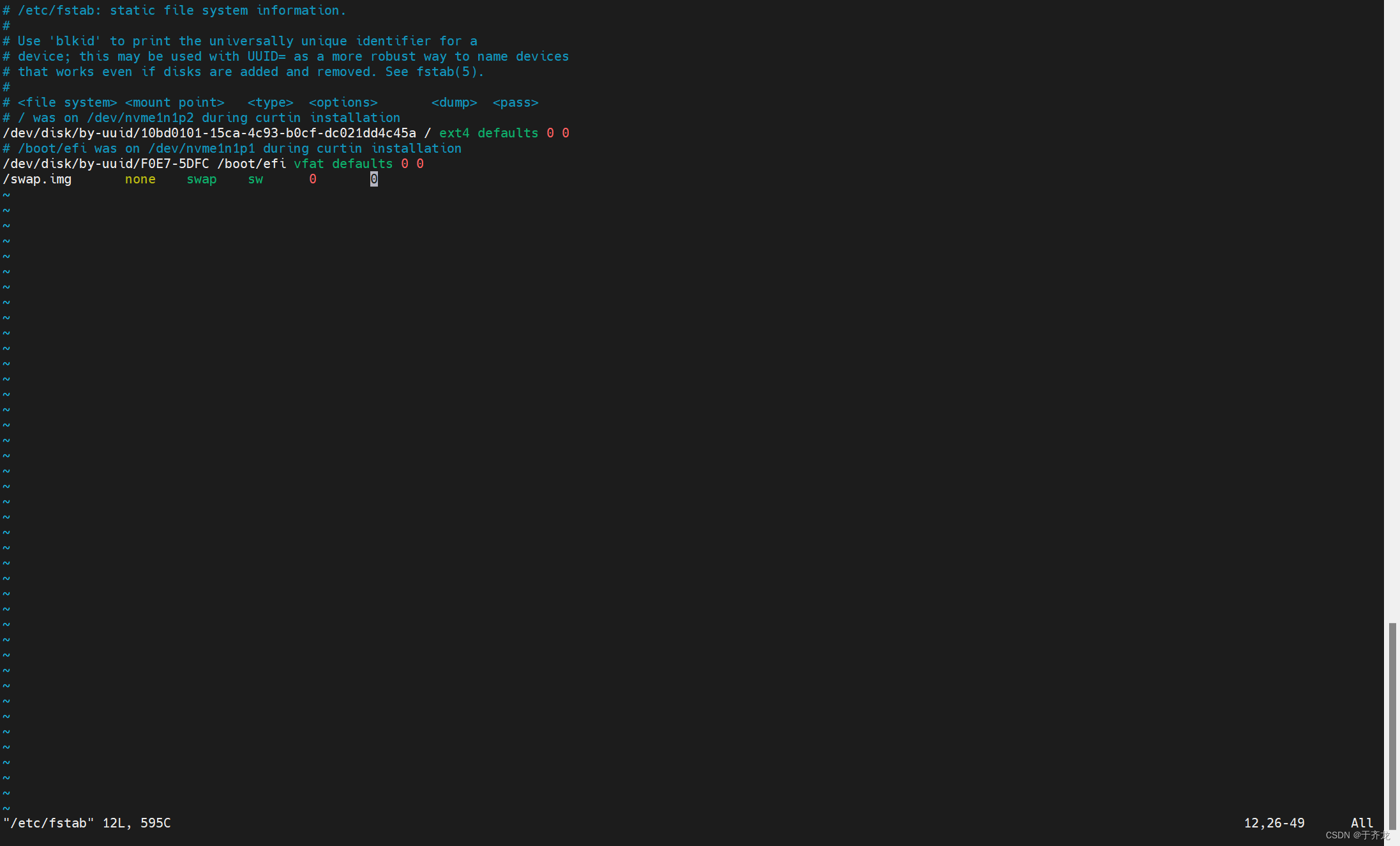
【Linux】进程(5):命令行参数
大家好,我是苏貝,本篇博客带大家了解Linux进程(5):命令行参数,如果你觉得我写的还不错的话,可以给我一个赞👍吗,感谢❤️ 目录 (A)为什么要有命令…...

vue2+antv/x6实现er图
效果图 安装依赖 npm install antv/x6 --save 我目前的项目安装的版本是antv/x6 2.18.1 人狠话不多,直接上代码 <template><div class"er-graph-container"><!-- 画布容器 --><div ref"graphContainerRef" id"gr…...

如何在XDMA中查看LTSSM状态机
简介 经常会遇到PCIe不能识别的问题,到底怎么去定位。本文以XDMA 为例,一方面复习下LTSSM状态机,一方面描述下如何通过FPGA的XDMA查看这个状态机 技术名词 LTSSM是一种常用于PCI Express(PCIe)接口的状态机…...

调用支付宝接口响应40004 SYSTEM_ERROR问题排查
在对接支付宝API的时候,遇到了一些问题,记录一下排查过程。 Body:{"datadigital_fincloud_generalsaas_face_certify_initialize_response":{"msg":"Business Failed","code":"40004","sub_msg…...

【SpringBoot】100、SpringBoot中使用自定义注解+AOP实现参数自动解密
在实际项目中,用户注册、登录、修改密码等操作,都涉及到参数传输安全问题。所以我们需要在前端对账户、密码等敏感信息加密传输,在后端接收到数据后能自动解密。 1、引入依赖 <dependency><groupId>org.springframework.boot</groupId><artifactId...

JVM垃圾回收机制全解析
Java虚拟机(JVM)中的垃圾收集器(Garbage Collector,简称GC)是用于自动管理内存的机制。它负责识别和清除不再被程序使用的对象,从而释放内存空间,避免内存泄漏和内存溢出等问题。垃圾收集器在Ja…...

oracle与MySQL数据库之间数据同步的技术要点
Oracle与MySQL数据库之间的数据同步是一个涉及多个技术要点的复杂任务。由于Oracle和MySQL的架构差异,它们的数据同步要求既要保持数据的准确性和一致性,又要处理好性能问题。以下是一些主要的技术要点: 数据结构差异 数据类型差异ÿ…...

企业如何增强终端安全?
在数字化转型加速的今天,企业的业务运行越来越依赖于终端设备。从员工的笔记本电脑、智能手机,到工厂里的物联网设备、智能传感器,这些终端构成了企业与外部世界连接的 “神经末梢”。然而,随着远程办公的常态化和设备接入的爆炸式…...
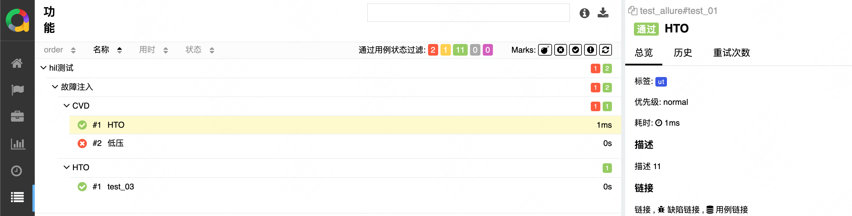
初学 pytest 记录
安装 pip install pytest用例可以是函数也可以是类中的方法 def test_func():print()class TestAdd: # def __init__(self): 在 pytest 中不可以使用__init__方法 # self.cc 12345 pytest.mark.api def test_str(self):res add(1, 2)assert res 12def test_int(self):r…...

人工智能(大型语言模型 LLMs)对不同学科的影响以及由此产生的新学习方式
今天是关于AI如何在教学中增强学生的学习体验,我把重要信息标红了。人文学科的价值被低估了 ⬇️ 转型与必要性 人工智能正在深刻地改变教育,这并非炒作,而是已经发生的巨大变革。教育机构和教育者不能忽视它,试图简单地禁止学生使…...

Web中间件--tomcat学习
Web中间件–tomcat Java虚拟机详解 什么是JAVA虚拟机 Java虚拟机是一个抽象的计算机,它可以执行Java字节码。Java虚拟机是Java平台的一部分,Java平台由Java语言、Java API和Java虚拟机组成。Java虚拟机的主要作用是将Java字节码转换为机器代码&#x…...

LangFlow技术架构分析
🔧 LangFlow 的可视化技术栈 前端节点编辑器 底层框架:基于 (一个现代化的 React 节点绘图库) 功能: 拖拽式构建 LangGraph 状态机 实时连线定义节点依赖关系 可视化调试循环和分支逻辑 与 LangGraph 的深…...
自然语言处理——文本分类
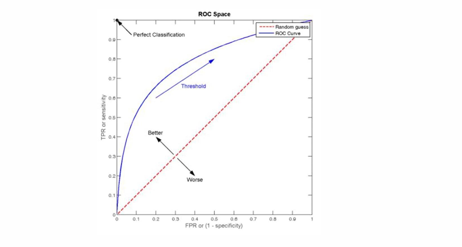
文本分类 传统机器学习方法文本表示向量空间模型 特征选择文档频率互信息信息增益(IG) 分类器设计贝叶斯理论:线性判别函数 文本分类性能评估P-R曲线ROC曲线 将文本文档或句子分类为预定义的类或类别, 有单标签多类别文本分类和多…...