【Neural signal processing and analysis zero to hero】- 2
Nonstationarities and effects of the FT
course from youtube: 传送地址


why we need extinguish stationary and non-stationary signal, because most of neural signal is non-stationary.

Welch’s method for smooth spectral decomposition
Full FFT method
you can see there are a lot of non stationarity x’ and temporal dynamics in this time domain signal so for example here you see when you look in the power spectrum you see very clearly that there is a peak at this frequency range and you know I don’t have the labels in here but this is somewhere around 40 to 50 Hertz so you see that there is a peak in the gamma somewhere around 40 to 50 Hertz so you see that there is a peak in the gamma frequency range here however just from looking at this Fourier transform result.

Welch’s method
 that is generally the result of Welch’s method it’s going to smooth out the power spectrum quite a bit


The filter-Hilbert time-frequency method
we have a signal that happens to be a Morley wavelet, there is only a real valued Morley wavelet. so the amplitude get split between the positive and the negative frequencies.

this actually is a complex valued signal so when you take the Hilbert transform of a real valued signal the output is in fact a complex valued signal so it has a real part and an imaginary part the real part is in green the imaginary part is an orange dashed line so why does this happen and how does the Hilbert transform at work well the way that the Hilbert transform is implemented in computers is often something like this now you look at frequency graph and this looks familiar this is the power spectrum of the complex morley wavelet. but that’s actually not what we created what we created was the Hilbert transform of a real valued wavelet and in fact what the Hilbert transform does is to take the FFT of the signal which is this go into the frequency domain 0 out all of the negative frequencies double the amplitudes of the positive frequencies and then take the inverse Fourier transform .
so what happens when you do that you know you go from wavelet from a real-valued signal into the frequency domain(bottom left) you will blitter 8 the negative frequencies double the amplitudes of the positive frequencies(bottom right) and then take the inverse Fourier transform that ends up giving us a complex valued wavelet(top right).

the goal of the Hilbert transform is not a complex valued signal also called an analytic signal that we can use to extract power or amplitude and phase information in addition to the real part of the signal so application of the Hilbert transform it converts a real valued signal into a complex valued analytic signal this result as it turns out is analogous to the result of complex more late wavelet convolution.


because of this really really important point and that is that the power and phase at each single time point resulting from the Hilbert transform come from the frequency that has the most power at that single time point. so therefore the output of the Hilbert transform is interpretable only for narrowband signals so that means that you shouldn’t apply the Hilbert to narrowband data but of course EEG and LFP our broadband phenomenon they have energy at a whole range of frequencies.

so what is the solution what do we do is to filter the data first so we apply a filter to the data that gets us from our original signal which is broadband to a filtered signal which is narrowband and then you can apply the Hilbert transform to this narrowband filtered signal.

Designing FIR bandpass filters
FIR(finite impulse response).
you have six data points, you need one at 0 that’s for DC and you need one at 1 and that’s for Nyquist and the you have four other points and these defines the shape of the filter in the frequency domain so these two points(top two) would correspond to the cut-offs that you are interested in. other tow points at axis called transition zone.

the idea of having a transition zone like this is that you don’t want to specify the filter with perfect edges you don’t want a sharp edge in the frequency domain and the reason why is because that will introduce or sharp edges in the frequency domain when you take the inverse Fourier transform that sharp edge that’s going to produce a lot of ripple effects in the time domain which can introduce artefactual oscillations.


The Short-time Fourier transform
Fourier transform as computing the dot product between this kernel and this entire signal and then so we use as a pivot to start talking about wavelets and convolution.
we can focus the analysis on one specific time window, so come up with the solution of taking this kernel and sliding it along the data but you might also have come up with a solution of instead of doing the Fourier transform on the entire signal you only do the a Fourier transform on one little segment of the signal.

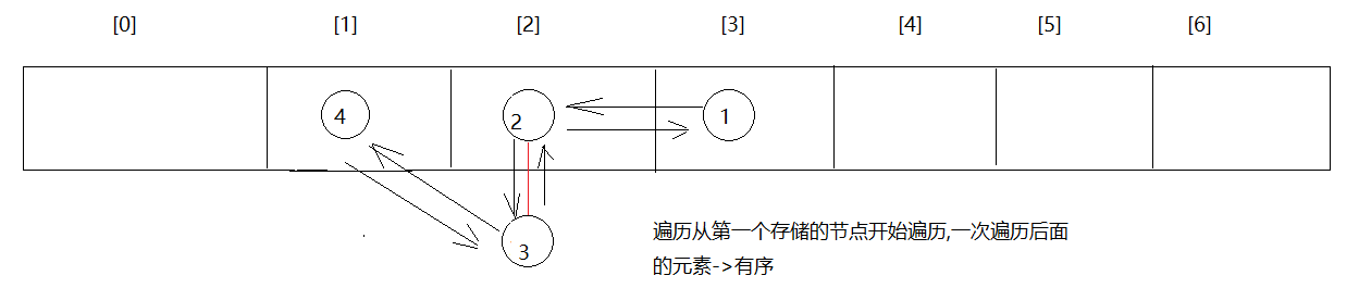
here is a time domain signal and then what we do is we cut out one snippet one epoch of this signal and that gives us a smaller signal that looks like the second graph, it gets tapered to attenuate the edges at the beginning and at the end.
we take the Fourier transform of the tapered version of the signal and then compute the power spectrum. then you take this power spectrum and you rotate it and color it, so in the second graph, frequency is on the x axis and power is on the y axis. in the second graph frequency is on the y axis and color is like z axis represent power. so we get one column in this time frequency matrix and what you do is take this window of time and you slide it over by hundred milliseconds or maybe 50 milliseconds.

one interesting difference between the short time Fourier transform and wavelet convolution:
wavelet convolution we build up the time frequency plane one frequency at a time for all time points and here with short time Fourier transform we building up the time frequency plane one time point at a time or on time chunk at a time over all frequencies at once. and then we’re looping over the different time points.
Comparing wavelet, filter-Hilbert, and STFFT


The multitaper method
if you have data are really non-time-locked, then they would be lost in the trail averaging, so what we want to do is have a method that is more robust to these temporal jitters essentially by smoothing over frequency and over time to allow you to identify these four features and averaged them together .

how do we average across these larger time windows well it worked by starting from these things called sleep tapers. these tapers are all orthogonal to each other so they are all mutually uncorrelated, so if you use these tapers on the same data they are going to highlight different features.

how does the multi taper method work well we start with our snippet of data, you take this first sleepy and taper and element-wise multiplication. and that’s going to give you a resulting time series that looks like this. and then move to the next taper, and we obtained a different one, we obtained four different time series.

now what we do is take the Fourier transform from each of these individual tapered time series and then extract power that gives you four different power spectra.

then we just average them together and that gives us one power spectrum and this corresponds to the multi taper estimate of the spectrum of the data snippet in
or using these different tapers and you can contrast this with a normal Fourier transform which would look like this so this is just the power spectrum from regular Fourier transform of the same data snippet so this spectrum and this spectrum come from exactly the same data these have been pushed through the multi taper method and this is just one FFT。
what you can see here is that the kind of prominent features of the spectrum are preserved and even a bit enhanced they are smooth in this spectrum but what you lose from the multi taper spectrum is kind of the finer details of the spectrum.


With-subject, cross-trail regression
Time-frequency brain-behavior correlations
we can do many trails for one subject, and we plot behavior-brain relationship graph, we want to fit a line taht goes through this blue dots.

this is a map that not a time frequency graph, all though the x axis is time and the y axis is frequency, but the color is corresponds to a correlation coefficient, so what you see is the energy over trails is related to the different reaction times over different trails.

the problem is how do we go about implementing this in an intelligent way. so we’re gonna do that using statistics and using the framework of the general linear model often abbreviated GLM.

Temporal resolution vs. precision

for wavelet convolution and filter Hilbert the time frequency analysis does not change the temporal resolution so if you have your data recorded at a kilohertz and then you do a wavelet convolution for time frequency analysis, the results of time frequency analysis are still at one kilohertz. you haven’t loss any time point, however what you done is reduce the temporal precision.
why? the answer is that it had to do with the amount of smoothing that gets imposed by the wavelet pr the filtering.

Separating phase-locked from non-phase-locked activity
we call a signal phased if the exact timing and also the phase time series is the same on every trail and therefore it survives trail averaging and we call a signal component non phase locked if the phase and exact timing is variable on different trails.
sometimes in the literature people call this evoked and induced.


for example, the blue line is ERP, the green is original signal, so the orange line is Non-phase-locked = Total - erp, then you can apply your time frequency analysis to this orange line, that will give you the time frequency power of the non phase-locked part of the signal.
the second graph, we can see the erp is small, so we don’t actually removing that much from the signal trail data, so separating out the erp or the phase-locked in the non phase-locked part of the signal is sample to do one thing: subtracting the ERP from the total signal that has to be done not only separately for each channel of course but also separately for each experiment condition so if you have an experiment with multiple different kinds of conditions different experiment conditions then you want to subtract compute and subtract the ERP separately for each condition for each single trial that comes from that condition that’s important to prevent any differences in the ERP from infecting the from introducing artificial differences in the total or the non phase-locked part of the signal.

after separating, you can make several time frequency plots and look like this.

Edge effects, buffer zones, and data epoch length
these red demons here on the side all the way on the left and all the way on the right these are edge effects they’re artifacts and they are contaminating their overriding the other signals the other features that are actually happening in the EEG data.

where do edge effects come from?
imagine if something like this is in your data then you’re going to get this now this is kind of as expected this isn’t really wrong. this is the correct answer however these edge effects can be so large that they will overwhelm whatever is the time frequency dynamics that are happening in the signal obviously there’s nothing happening in this signal but you can imagine that if this kind of an edge is superimposed on top of your EEG signal that this is going to be really difficult.
this is going to add an artifact that’s going to make it difficult to interpret what’s actually happening endogenously in a signal that was coming from the brain.

the solution is to accept the edge effects will be present and you just make sure that those edge effects are not going to contaminate the time windows that you are interested in.
so it related to cutting your epoch so cutting you continuous data into epochs.

one of the initial steps of pre-processing your data are to identify the timing of different events that happen in the experiment or if it’s spontaneous data or resting-state data. cut up the data into 2 seconds segment and then you cut epochs around each of these events and these from you trials.

so this would be the data frame from trail 1. but this still have edge effects

there are two solutions of dealing with edge effects what you can do instead is come up with one of two strategies to make sure that the edge effects are not going to contaminate the part of the signal that you want to interpret.
so the first solution is what I call the buffer zone approach so essentially what you want to do is make sure that you cut your epochs sufficiently long you want your time epochs your trials to be cut sufficiently wide such that the edge effects will totally subside. by the time you get to the time window that you are actually interested in. The only reason why the epochs are cut this long is so that the edge effects can fully subside both we get to the time period that I’m actually interested in.
the another approach is clipping approach, here the idea is that you estimate what parts of the data could be contaminated by edge effects and then you basically just remove those pixels from the time frequency plot in practice that can be done by setting the values to be n a n.

相关文章:
【Neural signal processing and analysis zero to hero】- 2
Nonstationarities and effects of the FT course from youtube: 传送地址 why we need extinguish stationary and non-stationary signal, because most of neural signal is non-stationary. Welch’s method for smooth spectral decomposition Full FFT method y…...

好用的AI搜索引擎
1. 360AI 搜索 访问 360AI 搜索: https://www.huntagi.com/sites/1706642948656.html 360AI 搜索介绍: 360AI 搜索,新一代智能答案引擎,值得信赖的智能搜索伙伴,为复杂搜索提供专业支持,解锁更相关、更全面的答案。AI…...
十、Java集合 ★ ✔(模块18-20)【泛型、通配符、List、Set、TreeSet、自然排序和比较器排序、Collections、可变参数、Map】
day05 泛型,数据结构,List,Set 今日目标 泛型使用 数据结构 List Set 1 泛型 1.1 泛型的介绍 ★ 泛型是一种类型参数,专门用来保存类型用的 最早接触泛型是在ArrayList,这个E就是所谓的泛型了。使用ArrayList时,只要给E指定某一个类型…...

阿里云开源 Qwen2-Audio 音频聊天和预训练大型音频语言模型
Qwen2-Audio由阿里巴巴集团Qwen团队开发,它能够接受各种音频信号输入,对语音指令进行音频分析或直接文本回复。与以往复杂的层次标签不同,Qwen2-Audio通过使用自然语言提示简化了预训练过程,并扩大了数据量。 喜好儿网 Qwen2-Au…...

SpringBoot集成MQTT实现交互服务通信
引言 本文是springboot集成mqtt的一个实战案例。 gitee代码库地址:源码地址 一、什么是MQTT MQTT(Message Queuing Telemetry Transport,消息队列遥测传输协议),是一种基于发布/订阅(publish/subscribe&…...

python实现插入排序、快速排序
python实现插入排序、快速排序 算法步骤: Python实现插入排序快速排序算法步骤: Python实现快速排序算法时间复杂度 插入排序是一种简单直观的排序算法。它的基本思想是通过构建有序序列,对于未排序数据,在已排序序列中从后向前扫…...
Spring Boot集成kudu快速入门Demo
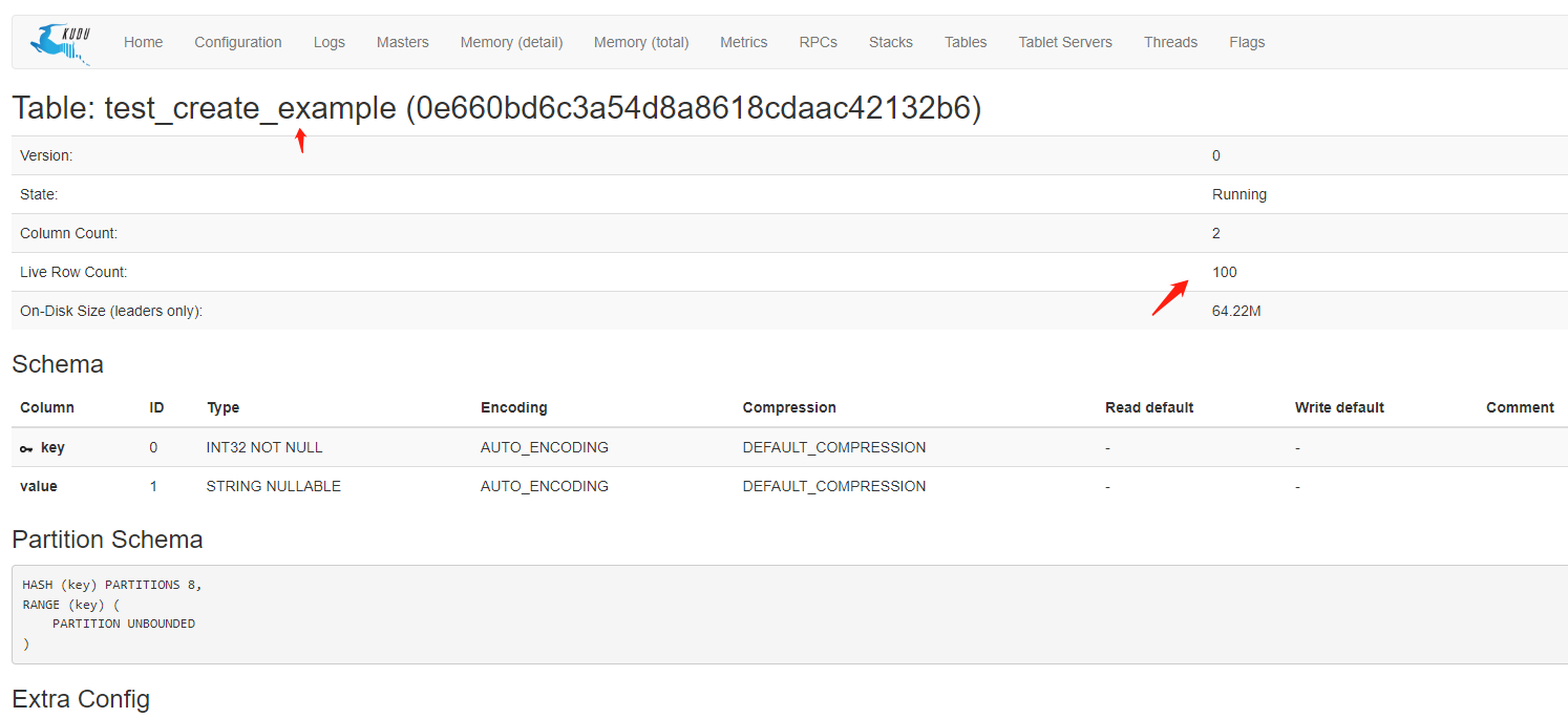
1.什么是kudu 在Kudu出现前,由于传统存储系统的局限性,对于数据的快速输入和分析还没有一个完美的解决方案,要么以缓慢的数据输入为代价实现快速分析,要么以缓慢的分析为代价实现数据快速输入。随着快速输入和分析场景越来越多&a…...

html超文本传输协议
在今天的Web开发学习中,我掌握了一些HTML和CSS的基础知识,下面我将分享我的学习笔记,帮助大家快速构建一个简单的Web界面。 一、HTML基础标签 1. 网站头 使用<title>标签定义网页的标题。 html <title>我的第一个网页</t…...

利用AI辅助制作ppt封面
如何利用AI辅助制作一个炫酷的PPT封面 标题使用镂空字背景替换为动态视频 标题使用镂空字 1.首先,新建一个空白的ppt页面,插入一张你认为符合主题的图片,占满整个可视页面。 2.其次,插入一个矩形,右键选择设置形状格式…...

【spring boot】初学者项目快速练手
一小时带你从0到1实现一个SpringBoot项目开发_哔哩哔哩_bilibili 一、简介 二、项目结构 三、代码结构 1.生成框架 Spring Initializr 快速生成一个初始的项目代码,会生成一个demo文件 打开intellj idea,导入demo文件 2.目录结构 源码都放在src-ma…...

Laravel+swoole 实现websocket长链接
需要使用 swoole 扩展 我使用的是 swoole 5.x start 方法启动服务 和 定时器 调整 listenQueue 定时器可以降低消息通讯延迟 定时器会自动推送队列里面的消息 testMessage 方法测试给指定用户推送消息 使用 laravel console 启动 <?phpnamespace App\Console\Comman…...

【C#】Array和List
C#中的List<T>和数组(T[])在某些方面是相似的,因为它们都是用来存储一系列元素的集合。然而,它们在功能和使用上有一些重要的区别: 数组(Array) 固定大小:数组的大小在声明时…...

SpringCloud网关的实现原理与使用指南
Spring Cloud网关是一个基于Spring Cloud的微服务网关,它是一个独立的项目,可以对外提供API接口服务,负责请求的转发和路由。本文将介绍Spring Cloud网关的实现原理和使用指南。 一、Spring Cloud网关的实现原理 Spring Cloud网关基于Spring…...
LabVIEW 与 PLC 通讯方式
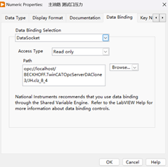
在工业自动化中,LabVIEW 与 PLC(可编程逻辑控制器)的通信至关重要,常见的通信方式包括 OPC、Modbus、EtherNet/IP、Profibus/Profinet 和 Serial(RS232/RS485)。这些通信协议各有特点和应用场景,…...

数据结构初阶·排序算法(内排序)
目录 前言: 1 冒泡排序 2 选择排序 3 插入排序 4 希尔排序 5 快速排序 5.1 Hoare版本 5.2 挖坑法 5.3 前后指针法 5.4 非递归快排 6 归并排序 6.1递归版本归并 6.2 非递归版本归并 7 计数排序 8 排序总结 前言: 目前常见的排序算法有9种…...

PL/SQL oracle上多表关联的一些记录
1.记录自己在PL/SQL上写的几张表的关联条件没有跑出来的一些优化 1. join后面跟上筛选条件 left join on t1.id t2.id and --- 带上分区字段,如 t1.month 202405, 操作跑不出来的一些问题,可能是数据量过大,未做分区过滤 2. 创建…...

Java.Net.UnknownHostException:揭开网络迷雾,解锁异常处理秘籍
在Java编程的浩瀚宇宙中,java.net.UnknownHostException犹如一朵不时飘过的乌云,让开发者在追求网络畅通无阻的道路上遭遇小挫。但别担心,今天我们就来一场说走就走的探险,揭秘这个异常的真面目,并手把手教你几招应对之…...

第十课:telnet(远程登入)
如何远程管理网络设备? 只要保证PC和路由器的ip是互通的,那么PC就可以远程管理路由器(用telnet技术管理)。 我们搭建一个下面这样的简单的拓扑图进行介绍 首先我们点击云,把云打开,点击增加 我们绑定vmn…...

【概率论三】参数估计:点估计(矩估计、极大似然法)、区间估计
文章目录 一. 点估计1. 矩估计法2. 极大似然法2.1. 似然函数2.2. 极大似然估计法 3. 评价估计量的标准3.1. 无偏性3.2. 有效性3.3. 一致性 二. 区间估计1. 区间估计的概念2. 正态总体参数的区间估计 参数估计讲什么 由样本来确定未知参数参数估计分为点估计与区间估计 一. 点估…...

自动化产线 搭配数据采集监控平台 创新与突破
自动化产线在现在的各行各业中应用广泛,已经是现在的生产趋势,不同的自动化生产设备充斥在各行各业中,自动化的设备会产生很多的数据,这些数据如何更科学化的管理,更优质的利用,就需要数据采集监控平台来完…...

实测AI读脸术:年龄性别识别效果展示,附详细使用教程
实测AI读脸术:年龄性别识别效果展示,附详细使用教程 1. 引言:一个开箱即用的人脸属性分析工具 你有没有想过,如果有一款工具,能像朋友一样看一眼照片,就告诉你里面人的大概年龄和性别,而且速度…...

陶晶驰TJC4832T135串口屏与STM32通信实战:从界面设计到数据交互全流程
陶晶驰TJC4832T135串口屏与STM32深度开发指南:从零构建工业级HMI交互系统 在工业控制、智能家居和物联网设备开发中,人机交互界面(HMI)的设计往往决定着产品的用户体验。陶晶驰TJC4832T135串口屏以其高性价比和稳定性能,成为STM32开发者常用的…...

Stable Yogi Leather-Dress-Collection企业应用:电商动漫服饰店铺主图AI生成标准化流程
Stable Yogi Leather-Dress-Collection企业应用:电商动漫服饰店铺主图AI生成标准化流程 你是不是也遇到过这样的烦恼?作为一家主打动漫风格皮衣的电商店铺,每次上新都要为几十款新品拍摄主图。找模特、租场地、请摄影师、后期修图……一套流…...

AI赋能机器人决策:使用快马Kimi模型生成智能清洁机器人行为树代码
最近在做一个模拟清洁机器人的小项目,想试试用AI来辅助生成它的“大脑”——也就是决策逻辑的代码。这个想法源于一个很实际的痛点:为机器人设计复杂的行为树或状态机时,既要考虑各种传感器输入的组合,又要确保逻辑清晰、易于维护…...

LangChain4j 赋能 SpringBoot:构建基于 Ollama 的本地智能对话服务
1. 为什么选择LangChain4j SpringBoot Ollama组合? 如果你正在寻找一种在Java生态中快速构建智能对话服务的方法,这个技术组合可能是目前最实用的选择。我最近在一个企业内部知识问答系统项目中实际采用了这套方案,发现它完美平衡了开发效率…...

计算机毕业设计springboot基于Java的高校毕业实习管理系统的设计与实现 基于SpringBoot的高校毕业生实习信息管理平台的设计与实现 基于Java技术的高校学生顶岗实习综合服务平台
计算机毕业设计springboot基于Java的高校毕业实习管理系统的设计与实现jctd2693 (配套有源码 程序 mysql数据库 论文) 本套源码可以在文本联xi,先看具体系统功能演示视频领取,可分享源码参考。随着高等教育的普及,每年有大量的学生…...

第一篇:从零搭建 Spring Boot 3 + Dubbo 3 + ZooKeeper 微服务实战
技术栈速览组件版本说明Spring Boot3.2.6基础框架Apache Dubbo3.3.4RPC 框架ZooKeeper3.9.2注册中心(Docker 部署)Curator5.xZK 客户端(由 Starter 管理)JDK17Spring Boot 3 最低要求项目目录结构先把整体结构了然于胸,…...
——附FDA合规性验证脚本)
临床队列分析总出错?(R tidyverse医学清洗模板大揭秘)——附FDA合规性验证脚本
第一章:临床队列分析出错的根源诊断与FDA合规性认知鸿沟临床队列分析在真实世界证据(RWE)生成中承担关键角色,但其结果偏差常源于底层数据治理缺陷与监管逻辑断层。当统计模型输出显著p值却无法通过FDA审评时,问题往往…...

基于IPv6与DDNS的远程办公解决方案:从路由器配置到Windows桌面控制
1. 为什么你需要IPv6DDNS:告别内网穿透的折腾 如果你和我一样,是个需要随时随地能连回家中电脑的上班族、开发者,或者只是想在外轻松管理家里网络设备的人,那你肯定没少为“远程访问”这件事头疼过。早几年,我们可能得…...

基于Matlab GUI的手势识别之旅
基于matlab gui的手势识别,导入手部图片,基于肤色模型的颜色分割,去噪,边缘提取,傅立叶算子特征提取,利用最小距离识别手势。最近在研究基于Matlab GUI的手势识别,觉得还挺有趣,来和…...