PyTorch搭建GNN(GCN、GraphSAGE和GAT)实现多节点、单节点内多变量输入多变量输出时空预测
目录
- I. 前言
- II. 数据集说明
- III. 模型
- 3.1 GCN
- 3.2 GraphSAGE
- 3.3 GAT
- IV. 训练与测试
- V. 实验结果
I. 前言
前面已经写了很多关于时间序列预测的文章:
- 深入理解PyTorch中LSTM的输入和输出(从input输入到Linear输出)
- PyTorch搭建LSTM实现时间序列预测(负荷预测)
- PyTorch中利用LSTMCell搭建多层LSTM实现时间序列预测
- PyTorch搭建LSTM实现多变量时间序列预测(负荷预测)
- PyTorch搭建双向LSTM实现时间序列预测(负荷预测)
- PyTorch搭建LSTM实现多变量多步长时间序列预测(一):直接多输出
- PyTorch搭建LSTM实现多变量多步长时间序列预测(二):单步滚动预测
- PyTorch搭建LSTM实现多变量多步长时间序列预测(三):多模型单步预测
- PyTorch搭建LSTM实现多变量多步长时间序列预测(四):多模型滚动预测
- PyTorch搭建LSTM实现多变量多步长时间序列预测(五):seq2seq
- PyTorch中实现LSTM多步长时间序列预测的几种方法总结(负荷预测)
- PyTorch-LSTM时间序列预测中如何预测真正的未来值
- PyTorch搭建LSTM实现多变量输入多变量输出时间序列预测(多任务学习)
- PyTorch搭建ANN实现时间序列预测(风速预测)
- PyTorch搭建CNN实现时间序列预测(风速预测)
- PyTorch搭建CNN-LSTM混合模型实现多变量多步长时间序列预测(负荷预测)
- PyTorch搭建Transformer实现多变量多步长时间序列预测(负荷预测)
- PyTorch时间序列预测系列文章总结(代码使用方法)
- TensorFlow搭建LSTM实现时间序列预测(负荷预测)
- TensorFlow搭建LSTM实现多变量时间序列预测(负荷预测)
- TensorFlow搭建双向LSTM实现时间序列预测(负荷预测)
- TensorFlow搭建LSTM实现多变量多步长时间序列预测(一):直接多输出
- TensorFlow搭建LSTM实现多变量多步长时间序列预测(二):单步滚动预测
- TensorFlow搭建LSTM实现多变量多步长时间序列预测(三):多模型单步预测
- TensorFlow搭建LSTM实现多变量多步长时间序列预测(四):多模型滚动预测
- TensorFlow搭建LSTM实现多变量多步长时间序列预测(五):seq2seq
- TensorFlow搭建LSTM实现多变量输入多变量输出时间序列预测(多任务学习)
- TensorFlow搭建ANN实现时间序列预测(风速预测)
- TensorFlow搭建CNN实现时间序列预测(风速预测)
- TensorFlow搭建CNN-LSTM混合模型实现多变量多步长时间序列预测(负荷预测)
- PyG搭建图神经网络实现多变量输入多变量输出时间序列预测
- PyTorch搭建GNN-LSTM和LSTM-GNN模型实现多变量输入多变量输出时间序列预测
- PyG Temporal搭建STGCN实现多变量输入多变量输出时间序列预测
- 时序预测中Attention机制是否真的有效?盘点LSTM/RNN中24种Attention机制+效果对比
- 详解Transformer在时序预测中的Encoder和Decoder过程:以负荷预测为例
- (PyTorch)TCN和RNN/LSTM/GRU结合实现时间序列预测
- PyTorch搭建Informer实现长序列时间序列预测
- PyTorch搭建Autoformer实现长序列时间序列预测
- PyTorch搭建GNN(GCN、GraphSAGE和GAT)实现多节点、单节点内多变量输入多变量输出时空预测
前边已经有两篇文章讲解了如何利用PyG搭建GNN以及GNN-LSTM进行时间序列预测,这两部分内容都只是针对多变量进行预测,即将每个变量当成一个节点,然后利用皮尔逊相关系数构建变量间的邻接矩阵。
上述过程有以下两个问题:
(1)不少人使用时不会安装PyG(后台经常有人询问如何安装PyG),这个其实不困难,具体安装命令为:
pip install torch_scatter torch_sparse torch_cluster torch_spline_conv torch-geometric -f https://data.pyg.org/whl/torch-1.10.0+cu113.html
使用时将命令中的torch-1.10.0+cu113.html换成自己的torch版本和CUDA版本即可。
(2)使用PyG有诸多限制,例如PyG中每个节点只能拥有单个变量序列。当然,可以将每个节点的多条变量序列用神经网络或者注意力机制等方式转换为一个变量序列,这里不再细说。
有不少人要求出一期多站点多变量预测,前期由于实习+秋招+毕设缠身,事情较多,所以没来得及写。现在有了一些空闲时间,因此在这篇文章里做一些详细的说明。
II. 数据集说明
本次使用的数据集为交通流量预测领域常见的PEMS系列数据集,包括PEMS03、PEMS04、PEMS07和PEMS08四个数据集。
其中,PEMS04是由307个探测器(节点数)每隔5分钟采集一次数据,共采集59天产生的交通流量数据;PEMS08是由170个探测器每隔5分钟采集一次,共采集62天产生的数据。每个探测器每次采集的数据包含三个维度的特征,分别为:流量、平均速度和平均占有率。因此,数据集的格式应该为一个矩阵,大小为num * num_nodes * 3,其中PSMS04的num=59*24*12=16992,num_nodes=307,而PEMS08的num=62*24*12=17856,num_nodes=170。PEMS03和PEMS07两个数据集中只包含流量这一个变量,二者的的大小分别为26208*358*1进和28224*883*1。
在这篇文章中,使用前2小时的数据预测未来半小时的数据,即历史24个时刻的多个变量预测未来6个时刻的多个变量。
数据处理代码与前面类似:
def nn_seq(args):seq_len = args.seq_lenbatch_size, pred_len = args.batch_size, args.pred_lenroot_path = os.path.abspath(os.path.dirname(os.getcwd()))file_name = args.file_namedata_path = root_path + "/data/" + file_name + "/"npz = np.load(data_path + file_name + ".npz")data = npz['data'] # lens num_nodes, in_featsprint(data.shape)# data = data[:2000]# 3表示:车流量、平均车速、平均车道占用率num_nodes = data.shape[1]# 加载邻接矩阵adj_data = pd.read_csv(data_path + file_name + ".csv")adj_data = adj_data[["from", "to"]].values.tolist()# 找出最大最小值all_elements = [element for row in adj_data for element in row]all_elements = list(set(all_elements))all_elements.sort()print(len(all_elements) == num_nodes)node_dict = dict(zip(all_elements, [x for x in range(num_nodes)]))# print(max_val, min_val)adj = torch.zeros((num_nodes, num_nodes))for src, dst in adj_data:src = node_dict[src]dst = node_dict[dst]adj[src, dst] = adj[dst, src] = 1## splittrain = data[:int(len(data) * 0.6)]val = data[int(len(data) * 0.6):int(len(data) * 0.8)]test = data[int(len(data) * 0.8):]# 归一化 要求在站点内部,对按照时间列进行归一化scalers = []for idx in range(num_nodes):cur_train = train[:, idx, :]cur_val = val[:, idx, :]cur_test = test[:, idx, :]scaler = MinMaxScaler()train[:, idx, :] = scaler.fit_transform(cur_train)val[:, idx, :] = scaler.transform(cur_val)test[:, idx, :] = scaler.transform(cur_test)scalers.append(scaler)def process(dataset, step_size, shuffle):# dataset: num num_nodes dimseq = []for i in tqdm(range(0, len(dataset) - seq_len - pred_len + 1, step_size)):x = dataset[i:i + seq_len]y = dataset[i + seq_len:i + seq_len + pred_len]# tensorx = torch.FloatTensor(x)y = torch.FloatTensor(y)seq.append((x, y))seq = MyDataset(seq)seq = DataLoader(dataset=seq, batch_size=batch_size, shuffle=shuffle, num_workers=0, drop_last=False)return seqDtr = process(train, step_size=1, shuffle=True)Val = process(val, step_size=1, shuffle=True)Dte = process(test, step_size=pred_len, shuffle=False)return Dtr, Val, Dte, adj, scalers
归一化时,由于不同站点间的数据没有太大关联,因此需要单独对每个站点内部的数据进行归一化,这里采用了MinMaxSacler归一化。
III. 模型
在这篇文章中将使用常见的三个GNN模型进行预测,即GCN、GraphSAGE和GAT。
图卷积网络(Graph Convolutional Network,GCN)是最早提出的图神经网络之一,GCN通过在图的邻域内进行信息聚合来学习节点的低维表示。具体来说,GCN利用了拉普拉斯矩阵的特征值分解,通过图傅里叶变换将卷积操作转换为频域上的滤波操作。GCN的核心公式为:
h ( l + 1 ) = σ ( D ~ − 1 2 A ~ D ~ − 1 2 h ( l ) W ( l ) ) h^{(l+1)} = \sigma(\tilde{D}^{-\frac{1}{2}} \tilde{A} \tilde{D}^{-\frac{1}{2}} h^{(l)} W^{(l)}) h(l+1)=σ(D~−21A~D~−21h(l)W(l))
其中, A ~ \tilde{A} A~是带有自环的邻接矩阵, D ~ \tilde{D} D~是对应的度矩阵, h ( l ) h^{(l)} h(l) 是第 l l l层的隐藏状态, W ( l ) W^{(l)} W(l)是权重矩阵, σ \sigma σ是激活函数。
GraphSAGE是由Hamilton等人在2017年提出的,旨在解决大规模图上的节点表示学习问题。GraphSAGE通过采样节点的邻居,并在局部邻域内进行信息聚合,从而生成节点表示。GraphSAGE支持多种聚合方法,包括 Mean Aggregator、LSTM Aggregator 和 Max Pooling Aggregator。GraphSAGE的核心公式为:
h i ( k + 1 ) = σ ( W f ( h i ( k ) , { h j ( k ) ∣ j ∈ N ( i ) } ) ) h_i^{(k+1)} = \sigma(W f(h_i^{(k)}, \{h_j^{(k)} | j \in \mathcal{N}(i)\})) hi(k+1)=σ(Wf(hi(k),{hj(k)∣j∈N(i)}))
其中 h i ( k ) h_i^{(k)} hi(k)是第 k k k层节点 i i i的隐藏状态, N ( i ) \mathcal{N}(i) N(i)是节点 i i i的邻居集合, f f f是聚合函数。GraphSAGE通过多层聚合操作,能够有效地捕捉节点的局部结构信息。
图注意力网络GAT(Graph Attention Networks)通过整合注意力机制实现了对图中不同邻居节点的动态加权。其主要创新之处在于,为每个邻接节点分配一个注意力得分,从而使模型可以聚焦于那些更为重要的邻近节点。GAT的核心公式为:
h i ( l + 1 ) = σ ( ∑ j ∈ N ( i ) α i j W h j ( l ) ) h_i^{(l+1)} = \sigma \left( \sum_{j \in \mathcal{N}(i)} \alpha_{ij} W h_j^{(l)} \right) hi(l+1)=σ j∈N(i)∑αijWhj(l)
其中 α i j \alpha_{ij} αij是节点 i i i和 j j j之间的注意力分数, W W W是权重矩阵。GAT通过自注意力机制,能够更好地捕捉节点之间的关系。
上述三种模型的原理十分简单,下边将依次介绍如何使用三种模型进行多站点、多变量输入、多变量输出的时空预测。
在进行模型讲解之前,先规定一下模型的输入和输出维度。在本文中,模型的输入尺寸为:batch_size * seq_len * num_nodes * in_feats,表示每个站点的多变量历史数据,输出为batch_size * pred_len * num_nodes * in_feats,表示多个站点未来的多变量数据。
3.1 GCN
GCN的代码实现十分优雅简洁,可以先看一下原作者的代码实现:
class GraphConvolution(Module):"""Simple GCN layer, similar to https://arxiv.org/abs/1609.02907"""def __init__(self, in_features, out_features, bias=True):super(GraphConvolution, self).__init__()self.in_features = in_featuresself.out_features = out_featuresself.weight = Parameter(torch.FloatTensor(in_features, out_features))if bias:self.bias = Parameter(torch.FloatTensor(out_features))else:self.register_parameter('bias', None)self.reset_parameters()def reset_parameters(self):stdv = 1. / math.sqrt(self.weight.size(1))self.weight.data.uniform_(-stdv, stdv)if self.bias is not None:self.bias.data.uniform_(-stdv, stdv)def forward(self, input, adj):support = torch.mm(input, self.weightoutput = torch.spmm(adj, support)if self.bias is not None:return output + self.biaselse:return outputdef __repr__(self):return self.__class__.__name__ + ' (' \+ str(self.in_features) + ' -> ' \+ str(self.out_features) + ')'
可以看到,GCN的本质就是将归一化后的邻接矩阵和节点特征矩阵执行矩阵乘法,即(num_nodes, num_nodes) * (num_nodes, feats) -> (num_nodes, feats)。
因此,对于大小为batch_size * seq_len * num_nodes * in_feats的输入,可以直接对后两个维度进行计算。代码如下:
class GCNConv(nn.Module):def __init__(self, in_features, out_features, bias=True):super(GCNConv, self).__init__()self.in_features = in_featuresself.out_features = out_featuresself.weight = Parameter(torch.FloatTensor(in_features, out_features))if bias:self.bias = Parameter(torch.FloatTensor(out_features))else:self.register_parameter('bias', None)self.reset_parameters()def reset_parameters(self):stdv = 1. / math.sqrt(self.weight.size(1))self.weight.data.uniform_(-stdv, stdv)if self.bias is not None:self.bias.data.uniform_(-stdv, stdv)def forward(self, x, adj):support = torch.matmul(x, self.weight)# 输入的数据是x = b s n d, adj = n * noutput = torch.einsum("tn,bsnd->bstd", adj, support) # bsndif self.bias is not None:output + self.biasreturn output
具体来讲,首先将batch_size * seq_len * num_nodes * in_feats利用self.weight变成batch_size * seq_len * num_nodes * out_feats,然后再与归一化后的邻接矩阵相乘,这里用到了torch.einsum()函数来指定参与计算的维度。
接着,便可以基于GCNConv来定义用于多站点。多变量输入、多变量输出的时刻预测GCN模型:
class GCN(torch.nn.Module):def __init__(self, args):super(GCN, self).__init__()self.args = argsself.conv1 = GCNConv(args.in_feats, args.h_feats)self.conv2 = GCNConv(args.h_feats, args.out_feats)self.dropout = 0.5self.fcs = nn.ModuleList()for _ in range(args.in_feats):self.fcs.append(nn.Sequential(nn.Linear(args.seq_len * args.out_feats, args.out_feats),nn.ReLU(),nn.Linear(args.out_feats, args.pred_len)))def forward(self, x, adj):# bsndx = F.dropout(x, self.dropout, training=self.training)x = F.elu(self.conv1(x, adj))x = self.conv2(x, adj)# b s n d --> b s n 3x = x.permute(0, 2, 1, 3) # bnsdx = torch.flatten(x, start_dim=2) # bn s*dpred = []for idx in range(self.args.in_feats):sub_pred = self.fcs[idx](x) # b n pred_lenpred.append(sub_pred) # b pred_len 3pred = torch.stack(pred, dim=-1) # b n pred_len 3# 变成和y一样的维度,即b pred_len num_node 3pred = pred.permute(0, 2, 1, 3)return pred
该模型由2个GCN层和一个预测层组成。输入batch_size * seq_len * num_nodes * in_feats(以下简称bsni)经过两层GCN变成bsno。接着,为了预测所有站点的多个变量,采用多任务学习中的思路,每个变量使用一个线性层进行预测。
预测时,首先将bsno的进行维度交换变成bnso,与LSTM等模型类似,可以将所有时刻的隐状态展开变成一个bn(s*d),然后使用多个线性层得到多个bn(pred_len),然后将多个变量的预测值拼接变成bn(pred_len)(in_feats)。最后,为了与真实值的batch_size * pred_len * num_nodes * in_feats相匹配,需要交换1和2两个维度。
需要注意的是,forward中传入的邻接矩阵是归一化后的邻接矩阵,归一化操作可以参考如下代码:
def normalize_adj(adj):"""归一化邻接矩阵,适用于图卷积网络(GCN)。:param adj: 原始邻接矩阵,形状为 (N, N):return: 归一化后的邻接矩阵,形状为 (N, N)"""# 添加自环adj = adj + torch.eye(adj.size(0))# 计算度矩阵 Ddegree = adj.sum(1)# 计算 D 的逆平方根d_inv_sqrt = torch.pow(degree, -0.5)d_inv_sqrt[torch.isinf(d_inv_sqrt)] = 0 # 防止出现无穷大# 构建 D 的逆平方根矩阵d_mat_inv_sqrt = torch.diag(d_inv_sqrt)# 归一化邻接矩阵adj_normalized = d_mat_inv_sqrt @ adj @ d_mat_inv_sqrtreturn adj_normalized
3.2 GraphSAGE
GraphSAGE的本质是将一个节点的邻居节点聚合后再与自身进行拼接变换,单层代码实现如下:
class SAGEConv(nn.Module):def __init__(self, in_features, out_features):super(SAGEConv, self).__init__()self.in_features = in_featuresself.out_features = out_featuresself.proj = nn.Linear(in_features, out_features)self.out_proj = nn.Linear(2 * out_features, out_features)def forward(self, x, adj):# 假设有多个站点support = self.proj(x)# 输入的数据是x = b s n d, adj = n * n# 邻居平均 设定一个很小的正数epseps = torch.tensor(1e-8)# 计算每一行的和,并确保不会除以零row_sums = adj.sum(dim=1, keepdim=True)row_sums = torch.max(row_sums, eps)# 对每一行进行规范化normalized_adj = adj / row_sumsoutput = torch.einsum("tn,bsnd->bstd", normalized_adj, support) # bsnd# catcat_x = torch.cat((support, output), dim=-1) # bsn 2dz = self.out_proj(cat_x)# normz_norm = z.norm(p=2, dim=-1, keepdim=True)z_norm = torch.where(z_norm == 0, torch.tensor(1.).to(z_norm), z_norm)z = z / z_normreturn z
上述代码采用的是平均聚合。与GCN类似,可以搭建GraphSAGE如下:
class GraphSAGE(torch.nn.Module):def __init__(self, args):super(GraphSAGE, self).__init__()self.args = argsself.conv1 = SAGEConv(args.in_feats, args.h_feats)self.conv2 = SAGEConv(args.h_feats, args.out_feats)self.dropout = 0.5self.fcs = nn.ModuleList()for _ in range(args.in_feats):self.fcs.append(nn.Sequential(nn.Linear(args.seq_len * args.out_feats, args.out_feats),nn.ReLU(),nn.Linear(args.out_feats, args.pred_len)))def forward(self, x, adj):# bsnd# x = F.dropout(x, self.dropout, training=self.training)x = F.relu(self.conv1(x, adj))x = self.conv2(x, adj)# b s n d --> b s n 3x = x.permute(0, 2, 1, 3) # bnsdx = torch.flatten(x, start_dim=2) # bn s*dpred = []for idx in range(self.args.in_feats):sub_pred = self.fcs[idx](x) # b n pred_lenpred.append(sub_pred) # b pred_len 3pred = torch.stack(pred, dim=-1) # b n pred_len 3pred = pred.permute(0, 2, 1, 3)return pred
3.3 GAT
GAT的代码稍显复杂,其本质是将节点的特征和邻居特征进行拼接然后变换得到这条边上的权重,最后再对邻居的特征进行加权。这里可以先参考一下GitHub上的GAT代码:
class GraphAttentionLayer(nn.Module):"""Simple GAT layer, similar to https://arxiv.org/abs/1710.10903"""def __init__(self, in_features, out_features, dropout, alpha, concat=True):super(GraphAttentionLayer, self).__init__()self.dropout = dropoutself.in_features = in_featuresself.out_features = out_featuresself.alpha = alphaself.concat = concatself.W = nn.Parameter(torch.empty(size=(in_features, out_features)))nn.init.xavier_uniform_(self.W.data, gain=1.414)self.a = nn.Parameter(torch.empty(size=(2*out_features, 1)))nn.init.xavier_uniform_(self.a.data, gain=1.414)self.leakyrelu = nn.LeakyReLU(self.alpha)def forward(self, h, adj):Wh = torch.mm(h, self.W) # h.shape: (N, in_features), Wh.shape: (N, out_features)e = self._prepare_attentional_mechanism_input(Wh)zero_vec = -9e15*torch.ones_like(e)attention = torch.where(adj > 0, e, zero_vec)attention = F.softmax(attention, dim=1)attention = F.dropout(attention, self.dropout, training=self.training)h_prime = torch.matmul(attention, Wh)if self.concat:return F.elu(h_prime)else:return h_primedef _prepare_attentional_mechanism_input(self, Wh):# Wh.shape (N, out_feature)# self.a.shape (2 * out_feature, 1)# Wh1&2.shape (N, 1)# e.shape (N, N)Wh1 = torch.matmul(Wh, self.a[:self.out_features, :])Wh2 = torch.matmul(Wh, self.a[self.out_features:, :])# broadcast adde = Wh1 + Wh2.Treturn self.leakyrelu(e)def __repr__(self):return self.__class__.__name__ + ' (' + str(self.in_features) + ' -> ' + str(self.out_features) + ')'
上述代码使用了broadcast add技巧来得到每个节点与其他所有节点的权重,然后再使用adj来将不存在边的权重变成一个很小的负数。
基于上述思想,可以将本文的图注意力层定义如下:
class GraphAttentionLayer(nn.Module):def __init__(self, in_features, out_features, dropout, alpha, concat=True):super(GraphAttentionLayer, self).__init__()self.dropout = dropoutself.in_features = in_featuresself.out_features = out_featuresself.alpha = alphaself.concat = concatself.W = nn.Parameter(torch.empty(size=(in_features, out_features)))nn.init.xavier_uniform_(self.W.data, gain=1.414)self.a = nn.Parameter(torch.empty(size=(2*out_features, 1)))nn.init.xavier_uniform_(self.a.data, gain=1.414)self.leakyrelu = nn.LeakyReLU(self.alpha)def forward(self, h, adj):# bsnd nnWh = torch.matmul(h, self.W)e = self._prepare_attentional_mechanism_input(Wh) # bsnn# 掩码操作mask = (adj == 0)# 广播掩码矩阵mask = mask.unsqueeze(0).unsqueeze(0)mask = mask.expand_as(e)# 应用掩码e[mask] = -9e15e = F.softmax(e, dim=1)e = F.dropout(e, self.dropout, training=self.training)h_prime = torch.einsum("bstn,bsnd->bstd", e, Wh) # bsndif self.concat:return F.elu(h_prime)else:return h_primedef _prepare_attentional_mechanism_input(self, Wh):# Wh.shape (bsz, seq_len, N, out_feature)# self.a.shape (2 * out_feature, 1)# Wh1&2.shape (N, 1)# e.shape (bsz, seq_len, N, N)Wh1 = torch.matmul(Wh, self.a[:self.out_features, :])Wh2 = torch.matmul(Wh, self.a[self.out_features:, :])# broadcast add# 只是最后两个维度相加e = Wh1 + Wh2.permute(0, 1, 3, 2)return self.leakyrelu(e)def __repr__(self):return self.__class__.__name__ + ' (' + str(self.in_features) + ' -> ' + str(self.out_features) + ')'
区别在于:
- 其一,执行broadcast add时候,只是后两个维度进行操作(
e = Wh1 + Wh2.permute(0, 1, 3, 2)),即bsnd+bsdn。 - 得到attention矩阵大小为bsnn,而不是二维的nn。因此,同样需要进行广播来实现掩码操作。
最后,基于GATConv,可以搭建一个简易版本(不使用多头注意力机制)的GAT如下:
class GAT(torch.nn.Module):def __init__(self, args):super(GAT, self).__init__()self.args = argsalpha = 0.2self.dropout = args.dropoutself.conv1 = GraphAttentionLayer(args.in_feats,args.h_feats,dropout=self.dropout, alpha=alpha, concat=False)self.conv2 = GraphAttentionLayer(args.h_feats,args.out_feats,dropout=self.dropout, alpha=alpha, concat=False)self.fcs = nn.ModuleList()for _ in range(args.in_feats):self.fcs.append(nn.Sequential(nn.Linear(args.seq_len * args.out_feats, args.out_feats),nn.ReLU(),nn.Linear(args.out_feats, args.pred_len)))def forward(self, x, adj):# bsndx = F.dropout(x, self.dropout, training=self.training)x = F.elu(self.conv1(x, adj))x = self.conv2(x, adj)# b s n d --> b s n 3x = x.permute(0, 2, 1, 3) # bnsdx = torch.flatten(x, start_dim=2) # bn s*dpred = []for idx in range(self.args.in_feats):sub_pred = self.fcs[idx](x) # b n pred_lenpred.append(sub_pred) # b pred_len 3pred = torch.stack(pred, dim=-1) # b n pred_len 3# 变成和y一样的维度,即b pred_len num_node 3pred = pred.permute(0, 2, 1, 3)return pred
当然,也可以使用多头注意力机制:
class GAT(nn.Module):def __init__(self, args):super(GAT, self).__init__()self.args = argsself.dropout = args.dropoutalpha = 0.2self.attentions = nn.ModuleList()for _ in range(args.heads):layer = GraphAttentionLayer(args.in_feats, args.h_feats, dropout=self.dropout, alpha=alpha, concat=True)self.attentions.append(layer)self.out_att = GraphAttentionLayer(args.h_feats * args.heads,args.out_feats,dropout=self.dropout, alpha=alpha, concat=False)# fcself.fcs = nn.ModuleList()for _ in range(args.in_feats):self.fcs.append(nn.Sequential(nn.Linear(args.seq_len * args.out_feats, args.out_feats),nn.ReLU(),nn.Linear(args.out_feats, args.pred_len)))def forward(self, x, adj):x = F.dropout(x, self.dropout, training=self.training)x = torch.cat([att(x, adj) for att in self.attentions], dim=-1)x = F.dropout(x, self.dropout, training=self.training)x = self.out_att(x, adj)# b s n d --> b s n 3x = x.permute(0, 2, 1, 3) # bnsdx = torch.flatten(x, start_dim=2) # bn s*dpred = []for idx in range(self.args.in_feats):sub_pred = self.fcs[idx](x) # b n pred_lenpred.append(sub_pred) # b pred_len 3pred = torch.stack(pred, dim=-1) # b n pred_len 3pred = pred.permute(0, 2, 1, 3)return pred
IV. 训练与测试
训练测试代码与之前差不太多,训练函数定义如下:
def train(args, Dtr, Val, adj, path, model_type):if model_type == "gcn":adj = normalize_adj(adj)model = GCN(args).to(device)elif model_type == "sage":model = GraphSAGE(args).to(device)elif model_type == "gat":model = GAT(args).to(device)else:raise ValueError("model_type has to be one of ('gcn', 'sage', 'gat')")adj = adj.to(device)loss_function = nn.MSELoss().to(device)optimizer = torch.optim.Adam(model.parameters(), lr=args.lr,weight_decay=args.weight_decay)scheduler = StepLR(optimizer, step_size=args.step_size, gamma=args.gamma)# trainingmin_epochs = 2best_model = Nonemin_val_loss = np.Inffor epoch in tqdm(range(args.epochs)):model.train()train_loss = []for (seq, label) in Dtr:optimizer.zero_grad()seq = seq.to(device)label = label.to(device) # b pred_len num_node 3pred = model(seq, adj) # b pred_len num_node 3# print(label.shape, pred.shape)loss = loss_function(pred, label)loss.backward()optimizer.step()train_loss.append(loss.item())scheduler.step()# validationval_loss = get_val_loss(args, model, Val, adj)if epoch + 1 >= min_epochs and val_loss < min_val_loss:min_val_loss = val_lossbest_model = copy.deepcopy(model)state = {'model': best_model.state_dict()}torch.save(state, path + '/models/' + model_type + '.pkl')print('epoch {:03d} train_loss {:.8f} val_loss {:.8f}'.format(epoch, np.mean(train_loss), val_loss))state = {'model': best_model.state_dict()}torch.save(state, path + '/models/' + model_type + '.pkl')
测试代码:
@torch.no_grad()
def test(args, Dte, adj, path, model_type, scalers):if model_type == "gcn":adj = normalize_adj(adj)model = GCN(args).to(device)elif model_type == "sage":model = GraphSAGE(args).to(device)elif model_type == "gat":model = GAT(args).to(device)else:raise ValueError("model_type has to be one of ('gcn', 'sage', 'gat')")model.load_state_dict(torch.load(path + '/models/' + model_type + '.pkl')['model'])adj = adj.to(device)y, pred = [], []for seq, label in Dte:seq = seq.to(device)y.append(label)sub_pred = model(seq, adj)  # b pred_len num_node 3pred.append(sub_pred.cpu())#y = torch.concat(y, dim=0)y = y.view(-1, y.size(2), y.size(3)).numpy()pred = torch.concat(pred, dim=0)  # num num_node 3pred = pred.view(-1, pred.size(2), pred.size(3)).numpy()# flatten# scalerfor idx in range(y.shape[1]):y[:, idx, :] = scalers[idx].inverse_transform(y[:, idx, :])pred[:, idx, :] = scalers[idx].inverse_transform(pred[:, idx, :])for idx in range(y.shape[1]):cur_y, cur_pred = y[:, idx, :], pred[:, idx, :]# 输出各种指标print('第{}个站点的指标为:'.format(idx + 1))maes, mses, rmses, mapes, r2s = get_metric(cur_y, cur_pred)print('mae:', maes)print('mse', mses)print('rmse:', rmses)print('mape:', mapes)print('r2:', r2s)# plotfor i in range(cur_y.shape[1]):plt.plot(cur_y[:, i], label="第{}个站点的第{}个变量的真实值".format(idx + 1, i + 1))plt.plot(cur_pred[:, i], label="第{}个站点的第{}个变量的预测值".format(idx + 1, i + 1))plt.legend()plt.show()
测试反归一化时注意在站点内进行归一化。
V. 实验结果
以PEMS04为例,下图展示了一些预测结果:

相关文章:
PyTorch搭建GNN(GCN、GraphSAGE和GAT)实现多节点、单节点内多变量输入多变量输出时空预测
目录 I. 前言II. 数据集说明III. 模型3.1 GCN3.2 GraphSAGE3.3 GAT IV. 训练与测试V. 实验结果 I. 前言 前面已经写了很多关于时间序列预测的文章: 深入理解PyTorch中LSTM的输入和输出(从input输入到Linear输出)PyTorch搭建LSTM实现时间序列…...

51单片机快速入门之数码管的拓展应用2024/10/15
51单片机快速入门之数码管的拓展应用 在前面的文章中,我们已经了解到数码管的基础应用,今天来讲讲拓展应用 我们知道单个数码管分为以下 但是当我们碰到 如下这种数码管的时候又应该如何去控制呢? 这里就不得不说其拓展应用之-----------扫描显示 扫描显示: 扫描显示,又称…...

vue 音频播放控件封装
<template> <div> <audio @timeupdate="updateProgress" controls ref="audioRef" style="display: none" > <source :src="audioUrl" type="audio/mpeg" /> 您的浏览器不支持音频播放 </audio&…...

秋招面试题记录
嵌入式软件开发 网上搜集的题目 1.Static关键词的作用? static 关键字有三个主要作用: 局部变量:在函数内部,static 局部变量只初始化一次,且在函数调用结束后仍然保留其值。全局变量/函数:在文件内部&a…...

金字塔流(Pyramid Flow): 用于生成人工智能长视频的新文本-视频开源模型
在 "生成式人工智能 "中的文本生成模型和图像生成模型大行其道之后,现在该是文本-视频模型大显身手的时候了,这个列表中的新模型就是 pyramid-flow-sd3,它是一个开源模型,用于从文本或图像生成长达 10 秒的视频…...

施磊C++ | 进阶学习笔记 | 5.设计模式
五、设计模式 文章目录 五、设计模式1.设计模式三大类型概述一、创建型设计模式二、结构型设计模式三、行为型设计模式 2.设计模式三大原则3.单例模式1.饿汉单例模式2.懒汉单例模式 4.线程安全的懒汉单例模式1.锁双重判断2.简洁的线程安全懒汉单例模式 5.简单工厂(Simple Facto…...

智绘城市地图:使用百度地图 API 实现智能定位
✨✨ 欢迎大家来访Srlua的博文(づ ̄3 ̄)づ╭❤~✨✨ 🌟🌟 欢迎各位亲爱的读者,感谢你们抽出宝贵的时间来阅读我的文章。 我是Srlua小谢,在这里我会分享我的知识和经验。&am…...

【稳定性】稳定性建设之变更管理
作者:京东物流 冯志文 背景 在软件开发和运维领域,变更管理是一个至关重要的环节。无论是对现有系统的改进、功能的增加还是修复漏洞,变更都是不可避免的。这些变更可能涉及到软件代码的修改、配置的调整、服务器的扩容、三方jar包的变更等等…...
c语言中字符串函数strlen,strcmp,strcpy,srtcat,strncpy,strncmp,strncat
1.strlen的使用和模拟实现 strlen 用来求字符串的长度,统计\0之前字符的个数。 模拟实现1:计数参数法 模拟实验2:指针方法 模拟实验3:递归方法 2,strcpy 的使用和模拟实现(拷贝字符串) char*…...

高级SQL技巧
高级SQL技巧涵盖了许多方面,包括但不限于窗口函数、递归查询、公共表表达式(CTEs)、子查询、集合操作、临时函数、日期时间操作、索引优化等。以下是对这些技巧的详细讲解和示例。 窗口函数 窗口函数是一种特殊的SQL函数,能够在…...

新大话西游图文架设教程
开始架设 1. 架设条件 新大话西游架设需要准备: linux 系统服务器,建议 CentOs 7.6或以上版本游戏源码,。 2. 安装宝塔面板 宝塔是一个服务器运维管理软件,安装命令: yum install -y wget && wget -O in…...

Maven 快速入门
Maven 快速入门 一、简介1、概述2、特点3、工作原理4、常用命令5、生命周期6、优缺点🎈 面试题 二、安装和配置1、安装2、环境配置3、命令测试是否安装成功4、功能配置5、idea配置本地 maven6、maven 工程依赖包查询网站 三、基于IDEA创建Maven工程1、maven 工程中的…...

OpenCV-人脸检测
文章目录 一、人脸检测流程二、关键方法三、代码示例四、注意事项 OpenCV是一个开源的计算机视觉和机器学习软件库,它提供了多种人脸检测方法,以下是对OpenCV人脸检测的详细介绍: 一、人脸检测流程 人脸检测是识别图像中人脸位置的过程&…...

【重磅升级】基于大数据的股票量化分析与预测系统
温馨提示:文末有 CSDN 平台官方提供的学长 QQ 名片 :) 1. 项目简介 伴随全球经济一体化和我国经济的快速发展,中国股票市场对世界经济的影响力不断攀升,中国股市已成为全球第二大股票交易市场。在当今的金融市场中,股票价格的波动…...

python全栈学习记录(二十四)元类、异常处理
元类、异常处理 文章目录 元类、异常处理一、元类1.元类控制类的实例化2.属性/方法的查找顺序3.单例 二、异常处理 一、元类 1.元类控制类的实例化 类的__call__方法会在产生的对象被调用时自动触发,args和kwargs就是调用实例时传入的参数,返回值是调用…...

Golang Slice扩容机制及注意事项
Golang Slice扩容机制及注意事项: 在 Go语言中,Slice(切片)是一种非常灵活且强大的数据结构,它是对数组的抽象,提供了动态数组的功能。Slice 的扩容机制是自动的,但了解其背后的原理对于编写高…...

华为OD机试 - 猜数字 - 暴力枚举(Python/JS/C/C++ 2024 E卷 100分)
华为OD机试 2024E卷题库疯狂收录中,刷题点这里 专栏导读 本专栏收录于《华为OD机试真题(Python/JS/C/C)》。 刷的越多,抽中的概率越大,私信哪吒,备注华为OD,加入华为OD刷题交流群,…...

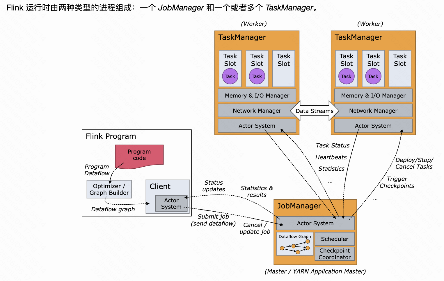
Flink触发器Trigger
前言 在 Flink 窗口计算模型中,数据先经过 WindowAssigner 分配窗口,然后再经过触发器 Trigger,Trigger 决定了一个窗口何时被 ProcessFunction 处理。每个 WindowAssigner 都有一个默认的 Trigger,如果默认的不满足需求…...

【操作系统的使用】Linux 系统环境变量与服务管理:设置与控制的艺术
文章目录 系统环境变量与服务管理:设置与控制的艺术一、系统环境变量的设置1.1 临时设置环境变量1.2 永久设置环境变量 二、服务启动类型的设置2.1 查看服务状态2.2 启动和停止服务2.3 设置服务的启动类型2.3.1 设置服务在启动时运行2.3.2 禁用服务在启动时运行2.3.…...

速盾:高防cdn配置中性能优化是什么?
高防CDN配置中的性能优化是指通过调整CDN配置以提升网站的加载速度、响应时间和用户体验。在进行性能优化时,需要考虑多个因素,包括CDN节点的选择和布置、缓存策略、缓存过期时间、预取和预加载、并发连接数和网络延迟等。 首先,CDN节点的选…...

Linux应用开发之网络套接字编程(实例篇)
服务端与客户端单连接 服务端代码 #include <sys/socket.h> #include <sys/types.h> #include <netinet/in.h> #include <stdio.h> #include <stdlib.h> #include <string.h> #include <arpa/inet.h> #include <pthread.h> …...

web vue 项目 Docker化部署
Web 项目 Docker 化部署详细教程 目录 Web 项目 Docker 化部署概述Dockerfile 详解 构建阶段生产阶段 构建和运行 Docker 镜像 1. Web 项目 Docker 化部署概述 Docker 化部署的主要步骤分为以下几个阶段: 构建阶段(Build Stage):…...

iOS 26 携众系统重磅更新,但“苹果智能”仍与国行无缘
美国西海岸的夏天,再次被苹果点燃。一年一度的全球开发者大会 WWDC25 如期而至,这不仅是开发者的盛宴,更是全球数亿苹果用户翘首以盼的科技春晚。今年,苹果依旧为我们带来了全家桶式的系统更新,包括 iOS 26、iPadOS 26…...

通过Wrangler CLI在worker中创建数据库和表
官方使用文档:Getting started Cloudflare D1 docs 创建数据库 在命令行中执行完成之后,会在本地和远程创建数据库: npx wranglerlatest d1 create prod-d1-tutorial 在cf中就可以看到数据库: 现在,您的Cloudfla…...

智能在线客服平台:数字化时代企业连接用户的 AI 中枢
随着互联网技术的飞速发展,消费者期望能够随时随地与企业进行交流。在线客服平台作为连接企业与客户的重要桥梁,不仅优化了客户体验,还提升了企业的服务效率和市场竞争力。本文将探讨在线客服平台的重要性、技术进展、实际应用,并…...

linux 下常用变更-8
1、删除普通用户 查询用户初始UID和GIDls -l /home/ ###家目录中查看UID cat /etc/group ###此文件查看GID删除用户1.编辑文件 /etc/passwd 找到对应的行,YW343:x:0:0::/home/YW343:/bin/bash 2.将标红的位置修改为用户对应初始UID和GID: YW3…...
《基于Apache Flink的流处理》笔记
思维导图 1-3 章 4-7章 8-11 章 参考资料 源码: https://github.com/streaming-with-flink 博客 https://flink.apache.org/bloghttps://www.ververica.com/blog 聚会及会议 https://flink-forward.orghttps://www.meetup.com/topics/apache-flink https://n…...
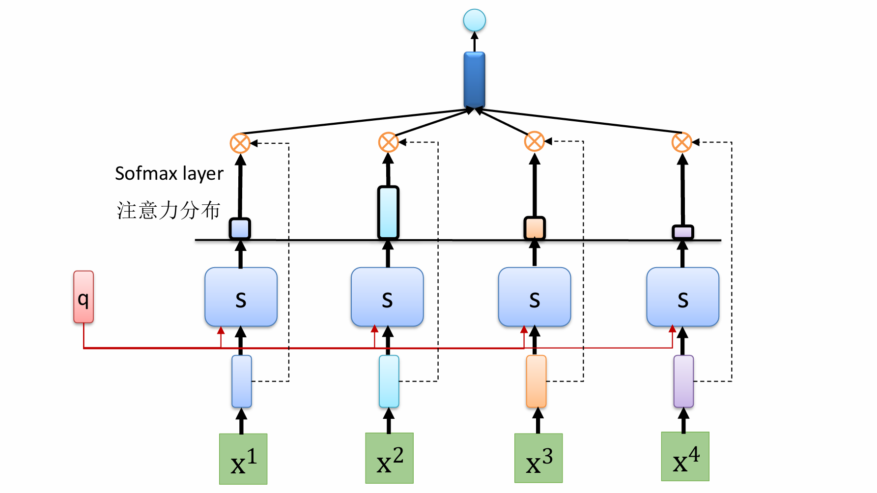
自然语言处理——循环神经网络
自然语言处理——循环神经网络 循环神经网络应用到基于机器学习的自然语言处理任务序列到类别同步的序列到序列模式异步的序列到序列模式 参数学习和长程依赖问题基于门控的循环神经网络门控循环单元(GRU)长短期记忆神经网络(LSTM)…...

稳定币的深度剖析与展望
一、引言 在当今数字化浪潮席卷全球的时代,加密货币作为一种新兴的金融现象,正以前所未有的速度改变着我们对传统货币和金融体系的认知。然而,加密货币市场的高度波动性却成为了其广泛应用和普及的一大障碍。在这样的背景下,稳定…...
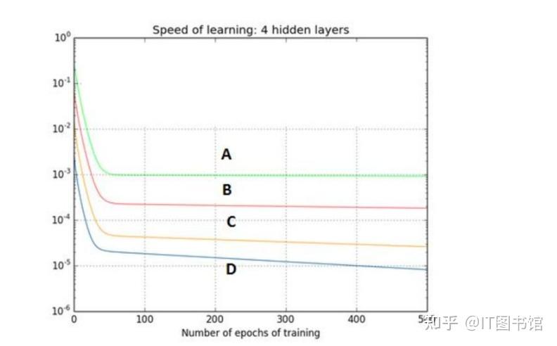
深度学习习题2
1.如果增加神经网络的宽度,精确度会增加到一个特定阈值后,便开始降低。造成这一现象的可能原因是什么? A、即使增加卷积核的数量,只有少部分的核会被用作预测 B、当卷积核数量增加时,神经网络的预测能力会降低 C、当卷…...