深度学习笔记之循环神经网络(九)GRU的反向传播过程
深度学习笔记之循环神经网络——GRU的反向传播过程
引言
上一节介绍了门控循环单元 ( Gate Recurrent Unit,GRU ) (\text{Gate Recurrent Unit,GRU}) (Gate Recurrent Unit,GRU),本节我们参照 LSTM \text{LSTM} LSTM反向传播的格式,观察 GRU \text{GRU} GRU的反向传播过程。
回顾: GRU \text{GRU} GRU的前馈计算过程

GRU \text{GRU} GRU的前馈计算过程表示如下:
为了后续的反向传播过程,将过程分解的细致一些。其中 Z ~ ( t ) , r ~ ( t ) \widetilde{\mathcal Z}^{(t)},\widetilde{r}^{(t)} Z (t),r (t)分别表示更新门、重置门的线性计算过程。
{ Z ~ ( t ) = W H ⇒ Z ⋅ h ( t − 1 ) + W X ⇒ Z ⋅ x ( t ) + b Z Z ( t ) = σ ( Z ~ ( t ) ) r ~ ( t ) = W H ⇒ r ⋅ h ( t − 1 ) + W X ⇒ r ⋅ x ( t ) + b r r ( t ) = σ ( r ~ ( t ) ) h ~ ( t ) = Tanh [ W H ⇒ H ~ ⋅ ( r ( t ) ∗ h ( t − 1 ) ) + W X ⇒ H ~ ⋅ x ( t ) + b H ~ ] h ( t ) = ( 1 − Z ( t ) ) ∗ h ( t − 1 ) + Z ( t ) ∗ h ~ ( t ) \begin{cases} \begin{aligned} & \widetilde{\mathcal Z}^{(t)} = \mathcal W_{\mathcal H \Rightarrow \mathcal Z} \cdot h^{(t-1)} + \mathcal W_{\mathcal X \Rightarrow \mathcal Z} \cdot x^{(t)} + b_{\mathcal Z} \\ & \mathcal Z^{(t)} = \sigma(\widetilde{\mathcal Z}^{(t)}) \\ & \widetilde{r}^{(t)} = \mathcal W_{\mathcal H \Rightarrow r} \cdot h^{(t-1)} + \mathcal W_{\mathcal X \Rightarrow r} \cdot x^{(t)} + b_{r} \\ & r^{(t)} = \sigma(\widetilde{r}^{(t)}) \\ & \widetilde{h}^{(t)} = \text{Tanh} \left[\mathcal W_{\mathcal H \Rightarrow \widetilde{\mathcal H}} \cdot (r^{(t)} * h^{(t-1)}) + \mathcal W_{\mathcal X \Rightarrow \widetilde{\mathcal H}} \cdot x^{(t)} + b_{\widetilde{\mathcal H}}\right] \\ & h^{(t)} = (1 -\mathcal Z^{(t)}) * h^{(t-1)} + \mathcal Z^{(t)} * \widetilde{h}^{(t)} \end{aligned} \end{cases} ⎩ ⎨ ⎧Z (t)=WH⇒Z⋅h(t−1)+WX⇒Z⋅x(t)+bZZ(t)=σ(Z (t))r (t)=WH⇒r⋅h(t−1)+WX⇒r⋅x(t)+brr(t)=σ(r (t))h (t)=Tanh[WH⇒H ⋅(r(t)∗h(t−1))+WX⇒H ⋅x(t)+bH ]h(t)=(1−Z(t))∗h(t−1)+Z(t)∗h (t)
场景设计
上述仅描述的是 GRU \text{GRU} GRU关于序列信息 h ( t ) ( t = 1 , 2 , ⋯ , T ) h^{(t)}(t=1,2,\cdots,\mathcal T) h(t)(t=1,2,⋯,T)的迭代过程。各时刻的输出特征以及损失函数于循环神经网络相同:
- 使用 Softmax \text{Softmax} Softmax激活函数,其输出结果作为模型对 t t t时刻的预测结果:
{ C ( t ) = W H ⇒ C ⋅ h ( t ) + b h y ^ ( t ) = Softmax ( C ( t ) ) \begin{cases} \mathcal C^{(t)} = \mathcal W_{\mathcal H \Rightarrow \mathcal C} \cdot h^{(t)} + b_{h} \\ \hat y^{(t)} = \text{Softmax}(\mathcal C^{(t)}) \end{cases} {C(t)=WH⇒C⋅h(t)+bhy^(t)=Softmax(C(t)) - 关于 t t t时刻预测结果 y ^ ( t ) \hat y^{(t)} y^(t)与真实分布 y ( t ) y^{(t)} y(t)之间的偏差信息使用交叉熵 ( CrossEntropy ) (\text{CrossEntropy}) (CrossEntropy)进行表示:
其中n Y n_{\mathcal Y} nY表示预测/真实分布的维数。
L ( t ) = L [ y ^ ( t ) , y ( t ) ] = − ∑ j = 1 n Y y j ( t ) log [ y ^ j ( t ) ] \mathcal L^{(t)} = \mathcal L \left[\hat y^{(t)},y^{(t)}\right] = - \sum_{j=1}^{n_\mathcal Y} y_j^{(t)} \log \left[\hat y_j^{(t)}\right] L(t)=L[y^(t),y(t)]=−j=1∑nYyj(t)log[y^j(t)] - 所有时刻交叉熵结果的累加和构成完整的损失函数 L \mathcal L L:
L = ∑ t = 1 T L ( t ) = ∑ t = 1 T L [ y ^ ( t ) , y ( t ) ] \begin{aligned} \mathcal L & = \sum_{t=1}^{\mathcal T} \mathcal L^{(t)}\\ & = \sum_{t=1}^{\mathcal T} \mathcal L \left[\hat y^{(t)},y^{(t)}\right] \end{aligned} L=t=1∑TL(t)=t=1∑TL[y^(t),y(t)]
反向传播过程
T \mathcal T T时刻的反向传播过程
以 T \mathcal T T时刻重置门 ∂ L ∂ W h ( T ) ⇒ Z ( T ) \begin{aligned}\frac{\partial \mathcal L}{\partial \mathcal W_{\mathcal h^{(\mathcal T)} \Rightarrow \mathcal Z^{(\mathcal T)}}}\end{aligned} ∂Wh(T)⇒Z(T)∂L的反向传播为例:
- 计算梯度 ∂ L ∂ L ( T ) \begin{aligned}\frac{\partial \mathcal L}{\partial \mathcal L^{(\mathcal T)}}\end{aligned} ∂L(T)∂L:
其中仅有L ( T ) \mathcal L^{(\mathcal T)} L(T)一项存在梯度,其余项均视作常数。
∂ L ∂ L ( T ) = ∂ ∂ L ( T ) [ ∑ t = 1 T L ( t ) ] = 0 + 0 + ⋯ + 1 = 1 \frac{\partial \mathcal L}{\partial \mathcal L^{(\mathcal T)}} = \frac{\partial}{\partial \mathcal L^{(\mathcal T)}} \left[\sum_{t=1}^{\mathcal T} \mathcal L^{(t)}\right] = 0 + 0 + \cdots + 1 = 1 ∂L(T)∂L=∂L(T)∂[t=1∑TL(t)]=0+0+⋯+1=1 - 计算梯度 ∂ L ( T ) ∂ C ( T ) \begin{aligned}\frac{\partial \mathcal L^{(\mathcal T)}}{\partial \mathcal C^{(\mathcal T)}}\end{aligned} ∂C(T)∂L(T):
关于Softmax \text{Softmax} Softmax激活函数与交叉熵组合的梯度描述,见循环神经网络—— Softmax \text{Softmax} Softmax函数的反向传播过程一节,这里不再赘述。
{ L ( T ) = − ∑ j = 1 n Y y j ( T ) log [ y ^ j ( T ) ] y ^ ( T ) = Softmax [ C ( T ) ] ⇒ ∂ L ( T ) ∂ C ( T ) = y ^ ( T ) − y ( T ) \begin{aligned} & \begin{cases} \mathcal L^{(\mathcal T)} = -\sum_{j=1}^{n_{\mathcal Y}}y_j^{(\mathcal T)} \log \left[\hat y_j^{(\mathcal T)}\right] \\ \hat y^{(\mathcal T)} = \text{Softmax}[\mathcal C^{(\mathcal T)}] \end{cases} \\ & \Rightarrow \frac{\partial \mathcal L^{(\mathcal T)}}{\partial \mathcal C^{(\mathcal T)}} = \hat y^{(\mathcal T)} - y^{(\mathcal T)} \end{aligned} {L(T)=−∑j=1nYyj(T)log[y^j(T)]y^(T)=Softmax[C(T)]⇒∂C(T)∂L(T)=y^(T)−y(T) - 继续计算梯度 ∂ C ( T ) ∂ h ( T ) \begin{aligned}\frac{\partial \mathcal C^{(\mathcal T)}}{\partial h^{(\mathcal T)}}\end{aligned} ∂h(T)∂C(T):
∂ C ( T ) ∂ h ( T ) = ∂ ∂ h ( T ) [ W H ⇒ C ⋅ h ( T ) + b h ] = W H ⇒ C \frac{\partial \mathcal C^{(\mathcal T)}}{\partial h^{(\mathcal T)}} = \frac{\partial}{\partial h^{(\mathcal T)}} \left[\mathcal W_{\mathcal H \Rightarrow \mathcal C} \cdot h^{(\mathcal T)} + b_{h}\right] = \mathcal W_{\mathcal H \Rightarrow \mathcal C} ∂h(T)∂C(T)=∂h(T)∂[WH⇒C⋅h(T)+bh]=WH⇒C
至此,关于梯度 ∂ L ∂ h ( T ) \begin{aligned}\frac{\partial \mathcal L}{\partial h^{(\mathcal T)}}\end{aligned} ∂h(T)∂L可表示为:
∂ L ∂ h ( T ) = ∂ L ∂ L ( T ) ⋅ ∂ L ( T ) ∂ C ( T ) ⋅ ∂ C ( T ) ∂ h ( T ) = 1 ⋅ [ W H ⇒ C ] T ⋅ ( y ^ ( T ) − y ( T ) ) \begin{aligned} \frac{\partial \mathcal L}{\partial h^{(\mathcal T)}} & = \frac{\partial \mathcal L}{\partial \mathcal L^{(\mathcal T)}} \cdot \frac{\partial \mathcal L^{(\mathcal T)}}{\partial \mathcal C^{(\mathcal T)}} \cdot \frac{\partial \mathcal C^{(\mathcal T)}}{\partial h^{(\mathcal T)}} \\ & = 1 \cdot \left[\mathcal W_{\mathcal H \Rightarrow \mathcal C}\right]^T \cdot (\hat y^{(\mathcal T)} - y^{(\mathcal T)}) \end{aligned} ∂h(T)∂L=∂L(T)∂L⋅∂C(T)∂L(T)⋅∂h(T)∂C(T)=1⋅[WH⇒C]T⋅(y^(T)−y(T))
观察:从 h ( T ) h^{(\mathcal T)} h(T)开始,从 h ( T ) ⇒ W h ( T ) ⇒ Z ( T ) h^{(\mathcal T)} \Rightarrow \mathcal W_{h^{(\mathcal T)} \Rightarrow \mathcal Z^{(\mathcal T)}} h(T)⇒Wh(T)⇒Z(T)的传播路径都有哪些。
只有唯一一条,其前馈计算路径表示为:
{ h ( t ) = ( 1 − Z ( t ) ) ∗ h ( t − 1 ) + Z ( t ) ∗ h ~ ( t ) Z ( t ) = σ ( Z ~ ( t ) ) Z ~ ( t ) = W H ⇒ Z ⋅ h ( t − 1 ) + W X ⇒ Z ⋅ x ( t ) + b Z \begin{cases} \begin{aligned} & h^{(t)} = (1 -\mathcal Z^{(t)}) * h^{(t-1)} + \mathcal Z^{(t)} * \widetilde{h}^{(t)} \\ & \mathcal Z^{(t)} = \sigma(\widetilde{\mathcal Z}^{(t)}) \\ & \widetilde{\mathcal Z}^{(t)} = \mathcal W_{\mathcal H \Rightarrow \mathcal Z} \cdot h^{(t-1)} + \mathcal W_{\mathcal X \Rightarrow \mathcal Z} \cdot x^{(t)} + b_{\mathcal Z} \end{aligned} \end{cases} ⎩ ⎨ ⎧h(t)=(1−Z(t))∗h(t−1)+Z(t)∗h (t)Z(t)=σ(Z (t))Z (t)=WH⇒Z⋅h(t−1)+WX⇒Z⋅x(t)+bZ
对应反向传播结果表示为:
∂ h ( T ) ∂ W h ( T ) ⇒ Z ( T ) = ∂ h ( T ) ∂ Z ( T ) ⋅ ∂ Z ( T ) ∂ Z ~ ( T ) ⋅ ∂ Z ~ ( T ) ∂ W h ( T ) ⇒ Z ( T ) = [ h ~ ( T ) − h ( T − 1 ) ] ⋅ [ Sigmoid ( Z ~ ( T ) ) ] ′ ⋅ h ( T − 1 ) \begin{aligned} \frac{\partial h^{(\mathcal T)}}{\partial \mathcal W_{h^{(\mathcal T)} \Rightarrow \mathcal Z^{(\mathcal T)}}} & = \frac{\partial h^{(\mathcal T)}}{\partial \mathcal Z^{(\mathcal T)}} \cdot \frac{\partial \mathcal Z^{(\mathcal T)}}{\partial \widetilde{\mathcal Z}^{(\mathcal T)}} \cdot \frac{\partial \widetilde{\mathcal Z}^{(\mathcal T)}}{\partial \mathcal W_{h^{(\mathcal T)} \Rightarrow \mathcal Z^{(\mathcal T)}}} \\ & = \left[\widetilde{h}^{(\mathcal T)} - h^{(\mathcal T - 1)}\right] \cdot \left[\text{Sigmoid}(\widetilde{\mathcal Z}^{(\mathcal T)})\right]' \cdot h^{(\mathcal T - 1)} \end{aligned} ∂Wh(T)⇒Z(T)∂h(T)=∂Z(T)∂h(T)⋅∂Z (T)∂Z(T)⋅∂Wh(T)⇒Z(T)∂Z (T)=[h (T)−h(T−1)]⋅[Sigmoid(Z (T))]′⋅h(T−1)
最终,关于 ∂ L ∂ W h ( T ) ⇒ Z ( T ) \begin{aligned}\frac{\partial \mathcal L}{\partial \mathcal W_{\mathcal h^{(\mathcal T)} \Rightarrow \mathcal Z^{(\mathcal T)}}}\end{aligned} ∂Wh(T)⇒Z(T)∂L的反向传播结果为:
这里更主要的是描述它的反向传播路径,它的具体展开在后续不再赘述。
∂ L ∂ W h ( T ) ⇒ Z ( T ) = ∂ L ∂ h ( T ) ⋅ ∂ h ( T ) ∂ W h ( T ) ⇒ Z ( T ) = { [ W H ⇒ C ] T ⋅ ( y ^ ( T ) − y ( T ) ) } ⋅ { [ h ~ ( T ) − h ( T − 1 ) ] ⋅ [ Sigmoid ( Z ~ ( T ) ) ] ′ ⋅ h ( T − 1 ) } \begin{aligned} \begin{aligned}\frac{\partial \mathcal L}{\partial \mathcal W_{\mathcal h^{(\mathcal T)} \Rightarrow \mathcal Z^{(\mathcal T)}}}\end{aligned} & = \frac{\partial \mathcal L}{\partial h^{(\mathcal T)}} \cdot \frac{\partial h^{(\mathcal T)}}{\partial \mathcal W_{h^{(\mathcal T)}\Rightarrow \mathcal Z^{(\mathcal T)}}} \\ & = \left\{\left[\mathcal W_{\mathcal H \Rightarrow \mathcal C}\right]^T \cdot (\hat y^{(\mathcal T)} - y^{(\mathcal T)})\right\} \cdot \left\{ \left[\widetilde{h}^{(\mathcal T)} - h^{(\mathcal T - 1)}\right] \cdot \left[\text{Sigmoid}(\widetilde{\mathcal Z}^{(\mathcal T)})\right]' \cdot h^{(\mathcal T - 1)}\right\} \end{aligned} ∂Wh(T)⇒Z(T)∂L=∂h(T)∂L⋅∂Wh(T)⇒Z(T)∂h(T)={[WH⇒C]T⋅(y^(T)−y(T))}⋅{[h (T)−h(T−1)]⋅[Sigmoid(Z (T))]′⋅h(T−1)}
T − 1 \mathcal T - 1 T−1时刻的反向传播路径
关于 T − 1 \mathcal T - 1 T−1时刻的重置门梯度 ∂ L ∂ W h ( T − 1 ) ⇒ Z ( T − 1 ) \begin{aligned} \frac{\partial \mathcal L}{\partial \mathcal W_{h^{(\mathcal T - 1)} \Rightarrow \mathcal Z^{(\mathcal T - 1)}}} \end{aligned} ∂Wh(T−1)⇒Z(T−1)∂L,它的路径主要包含两大类:
第一类路径:同 T \mathcal T T时刻路径,从对应的 L ( T − 1 ) \mathcal L^{(\mathcal T - 1)} L(T−1)直接传至 W h ( T − 1 ) ⇒ Z ( T − 1 ) \mathcal W_{h^{(\mathcal T - 1)}\Rightarrow \mathcal Z^{(\mathcal T - 1)}} Wh(T−1)⇒Z(T−1):
该路径与上述 T \mathcal T T时刻的路径类型相同,将对应的上标 T \mathcal T T改为 T − 1 \mathcal T - 1 T−1即可。
∂ L ( T − 1 ) ∂ W h ( T − 1 ) ⇒ Z ( T − 1 ) = ∂ L ( T − 1 ) ∂ h ( T − 1 ) ⋅ ∂ h ( T − 1 ) ∂ W h ( T − 1 ) ⇒ Z ( T − 1 ) \begin{aligned} \frac{\partial \mathcal L^{(\mathcal T - 1)}}{\partial \mathcal W_{h^{(\mathcal T - 1)} \Rightarrow \mathcal Z^{(\mathcal T - 1)}}} & = \frac{\partial \mathcal L^{(\mathcal T - 1)}}{\partial h^{(\mathcal T - 1)}} \cdot \frac{\partial h^{(\mathcal T - 1)}}{\partial \mathcal W_{h^{(\mathcal T - 1)} \Rightarrow \mathcal Z^{(\mathcal T - 1)}}} \end{aligned} ∂Wh(T−1)⇒Z(T−1)∂L(T−1)=∂h(T−1)∂L(T−1)⋅∂Wh(T−1)⇒Z(T−1)∂h(T−1)
第二类路径:重新观察 W h ( T − 1 ) ⇒ Z ( T − 1 ) \mathcal W_{h^{(\mathcal T - 1)}\Rightarrow \mathcal Z^{(\mathcal T - 1)}} Wh(T−1)⇒Z(T−1)只会出现在 Z ( T − 1 ) \mathcal Z^{(\mathcal T - 1)} Z(T−1)中,并且 Z ( T − 1 ) \mathcal Z^{(\mathcal T - 1)} Z(T−1)只会出现在 h ( T − 1 ) h^{(\mathcal T - 1)} h(T−1)中。因此:仅需要找出与 h ( T − 1 ) h^{(\mathcal T - 1)} h(T−1)相关的所有路径即可,最终都可以使用 ∂ h ( T − 1 ) ∂ W h ( T − 1 ) ⇒ Z ( T − 1 ) \begin{aligned}\frac{\partial h^{(\mathcal T - 1)}}{\partial \mathcal W_{h^{(\mathcal T - 1)} \Rightarrow \mathcal Z^{(\mathcal T - 1)}}}\end{aligned} ∂Wh(T−1)⇒Z(T−1)∂h(T−1)将梯度传递给 W h ( T − 1 ) ⇒ Z ( T − 1 ) \mathcal W_{h^{(\mathcal T - 1)} \Rightarrow \mathcal Z^{(\mathcal T - 1)}} Wh(T−1)⇒Z(T−1)。
其中‘第一类路径’就是其中一种情况。只不过它是从当前 T − 1 \mathcal T - 1 T−1时刻直接传递得到的梯度结果。而第二类路径我们关注从 T \mathcal T T时刻传递产生的梯度信息。
从 T ⇒ T − 1 \mathcal T \Rightarrow \mathcal T - 1 T⇒T−1时刻中,关于 h ( T − 1 ) h^{(\mathcal T - 1)} h(T−1)的梯度路径一共包含 4 4 4条:
- 第一条:通过 T \mathcal T T时刻 h ( T ) h^{(\mathcal T)} h(T)中的 h ( T − 1 ) h^{(\mathcal T - 1)} h(T−1)进行传递。
{ Forword : h ( T ) = ( 1 − Z ( T ) ) ∗ h ( T − 1 ) + Z ( T ) ∗ h ~ ( T ) Backward : ∂ L ( T ) ∂ W h ( T − 1 ) ⇒ Z ( T − 1 ) ⇒ ∂ L ( T ) ∂ h ( T ) ⋅ ∂ h ( T ) ∂ h ( T − 1 ) ⋅ ∂ h ( T − 1 ) ∂ W h ( T − 1 ) ⇒ Z ( T − 1 ) \begin{cases} \text{Forword : } h^{(\mathcal T)} = (1 -\mathcal Z^{(\mathcal T)}) * h^{(\mathcal T -1)} + \mathcal Z^{(\mathcal T)} * \widetilde{h}^{(\mathcal T)} \\ \quad \\ \text{Backward : }\begin{aligned} \frac{\partial \mathcal L^{(\mathcal T)}}{\partial \mathcal W_{h^{(\mathcal T - 1)} \Rightarrow \mathcal Z^{(\mathcal T - 1)}}} \Rightarrow \frac{\partial \mathcal L^{(\mathcal T)}}{\partial h^{(\mathcal T)}} \cdot \frac{\partial h^{(\mathcal T)}}{\partial h^{(\mathcal T - 1)}} \cdot \frac{\partial h^{(\mathcal T - 1)}}{\partial \mathcal W_{h^{(\mathcal T - 1)} \Rightarrow \mathcal Z^{(\mathcal T - 1)}}} \end{aligned} \end{cases} ⎩ ⎨ ⎧Forword : h(T)=(1−Z(T))∗h(T−1)+Z(T)∗h (T)Backward : ∂Wh(T−1)⇒Z(T−1)∂L(T)⇒∂h(T)∂L(T)⋅∂h(T−1)∂h(T)⋅∂Wh(T−1)⇒Z(T−1)∂h(T−1) - 第二条:通过 T \mathcal T T时刻 h ( T ) h^{(\mathcal T)} h(T)中的 Z ( T ) \mathcal Z^{(\mathcal T)} Z(T)向 h ( T − 1 ) h^{(\mathcal T-1)} h(T−1)进行传递。
{ Forward : { h ( T ) = ( 1 − Z ( T ) ) ∗ h ( T − 1 ) + Z ( T ) ∗ h ~ ( T ) Z ( T ) = σ [ W H ⇒ Z ⋅ h ( T − 1 ) + W X ⇒ Z ⋅ x ( T ) + b Z ] Backward : ∂ L ( T ) ∂ W h ( T − 1 ) ⇒ Z ( T − 1 ) ⇒ ∂ L ( T ) ∂ h ( T ) ⋅ ∂ h ( T ) ∂ Z ( T ) ⋅ ∂ Z ( T ) ∂ h ( T − 1 ) ⋅ ∂ h ( T − 1 ) ∂ W h ( T − 1 ) ⇒ Z ( T − 1 ) \begin{cases} \text{Forward : } \begin{cases} h^{(\mathcal T)} = (1 -\mathcal Z^{(\mathcal T)}) * h^{(\mathcal T -1)} + \mathcal Z^{(\mathcal T)} * \widetilde{h}^{(\mathcal T)} \\ \mathcal Z^{(\mathcal T)} = \sigma \left[\mathcal W_{\mathcal H \Rightarrow \mathcal Z} \cdot h^{(\mathcal T -1)} + \mathcal W_{\mathcal X \Rightarrow \mathcal Z} \cdot x^{(\mathcal T)} + b_{\mathcal Z}\right] \end{cases} \quad \\ \text{Backward : } \begin{aligned} \frac{\partial \mathcal L^{(\mathcal T)}}{\partial \mathcal W_{h^{(\mathcal T - 1)} \Rightarrow \mathcal Z^{(\mathcal T - 1)}}} \Rightarrow \frac{\partial \mathcal L^{(\mathcal T)}}{\partial h^{(\mathcal T)}} \cdot \frac{\partial h^{(\mathcal T)}}{\partial \mathcal Z^{(\mathcal T)}} \cdot \frac{\partial \mathcal Z^{(\mathcal T)}}{\partial h^{(\mathcal T - 1)}} \cdot \frac{\partial h^{(\mathcal T - 1)}}{\partial \mathcal W_{h^{(\mathcal T - 1)} \Rightarrow \mathcal Z^{(\mathcal T - 1)}}} \end{aligned} \end{cases} ⎩ ⎨ ⎧Forward : {h(T)=(1−Z(T))∗h(T−1)+Z(T)∗h (T)Z(T)=σ[WH⇒Z⋅h(T−1)+WX⇒Z⋅x(T)+bZ]Backward : ∂Wh(T−1)⇒Z(T−1)∂L(T)⇒∂h(T)∂L(T)⋅∂Z(T)∂h(T)⋅∂h(T−1)∂Z(T)⋅∂Wh(T−1)⇒Z(T−1)∂h(T−1) - 第三条:通过 T \mathcal T T时刻 h ( T ) h^{(\mathcal T)} h(T)中的 h ~ ( T ) \widetilde{h}^{(\mathcal T)} h (T)向 h ( T − 1 ) h^{(\mathcal T - 1)} h(T−1)进行传递。
{ Forward : { h ( T ) = ( 1 − Z ( T ) ) ∗ h ( T − 1 ) + Z ( T ) ∗ h ~ ( T ) h ~ ( T ) = Tanh [ W H ⇒ H ~ ⋅ ( r ( T ) ∗ h ( T − 1 ) ) + W X ⇒ H ~ ⋅ x ( T ) + b H ~ ] Backward : ∂ L ( T ) ∂ W h ( T − 1 ) ⇒ Z ( T − 1 ) ⇒ ∂ L ( T ) ∂ h ( T ) ⋅ ∂ h ( T ) ∂ h ~ ( T ) ⋅ h ~ ( T ) ∂ h ( T − 1 ) ⋅ ∂ h ( T − 1 ) ∂ W h ( T − 1 ) ⇒ Z ( T − 1 ) \begin{cases} \text{Forward : } \begin{cases} h^{(\mathcal T)} = (1 -\mathcal Z^{(\mathcal T)}) * h^{(\mathcal T -1)} + \mathcal Z^{(\mathcal T)} * \widetilde{h}^{(\mathcal T)} \\ \widetilde{h}^{(\mathcal T)} = \text{Tanh} \left[\mathcal W_{\mathcal H \Rightarrow \widetilde{\mathcal H}} \cdot (r^{(\mathcal T)} * h^{(\mathcal T -1)}) + \mathcal W_{\mathcal X \Rightarrow \widetilde{\mathcal H}} \cdot x^{(\mathcal T)} + b_{\widetilde{\mathcal H}}\right] \end{cases}\\ \quad \\ \text{Backward : } \begin{aligned} \frac{\partial \mathcal L^{(\mathcal T)}}{\partial \mathcal W_{h^{(\mathcal T - 1)} \Rightarrow \mathcal Z^{(\mathcal T - 1)}}} \Rightarrow \frac{\partial \mathcal L^{(\mathcal T)}}{\partial h^{(\mathcal T)}} \cdot \frac{\partial h^{(\mathcal T)}}{\partial \widetilde{h}^{(\mathcal T)}} \cdot \frac{\widetilde{h}^{(\mathcal T)}}{\partial h^{(\mathcal T - 1)}} \cdot \frac{\partial h^{(\mathcal T - 1)}}{\partial \mathcal W_{h^{(\mathcal T - 1)} \Rightarrow \mathcal Z^{(\mathcal T - 1)}}} \end{aligned} \end{cases} ⎩ ⎨ ⎧Forward : {h(T)=(1−Z(T))∗h(T−1)+Z(T)∗h (T)h (T)=Tanh[WH⇒H ⋅(r(T)∗h(T−1))+WX⇒H ⋅x(T)+bH ]Backward : ∂Wh(T−1)⇒Z(T−1)∂L(T)⇒∂h(T)∂L(T)⋅∂h (T)∂h(T)⋅∂h(T−1)h (T)⋅∂Wh(T−1)⇒Z(T−1)∂h(T−1) - 第四条:与第三条路径类似,只不过从 h ~ ( T ) \widetilde{h}^{(\mathcal T)} h (T)中的 r ( T ) r^{(\mathcal T)} r(T)向 h ( T − 1 ) h^{(\mathcal T - 1)} h(T−1)进行传递。
{ Forward : { h ( T ) = ( 1 − Z ( T ) ) ∗ h ( T − 1 ) + Z ( T ) ∗ h ~ ( T ) h ~ ( T ) = Tanh [ W H ⇒ H ~ ⋅ ( r ( T ) ∗ h ( T − 1 ) ) + W X ⇒ H ~ ⋅ x ( T ) + b H ~ ] r ~ ( T ) = W H ⇒ r ⋅ h ( T − 1 ) + W X ⇒ r ⋅ x ( T ) + b r Backward : ∂ L ( T ) ∂ W h ( T − 1 ) ⇒ Z ( T − 1 ) ⇒ ∂ L ( T ) ∂ h ( T ) ⋅ ∂ h ( T ) ∂ h ~ ( T ) ⋅ ∂ h ~ ( T ) ∂ r ( T ) ⋅ ∂ r ( T ) ∂ h ( T − 1 ) ⋅ ∂ h ( T − 1 ) ∂ W h ( T − 1 ) ⇒ Z ( T − 1 ) \begin{cases} \text{Forward : } \begin{cases} h^{(\mathcal T)} = (1 -\mathcal Z^{(\mathcal T)}) * h^{(\mathcal T -1)} + \mathcal Z^{(\mathcal T)} * \widetilde{h}^{(\mathcal T)} \\ \widetilde{h}^{(\mathcal T)} = \text{Tanh} \left[\mathcal W_{\mathcal H \Rightarrow \widetilde{\mathcal H}} \cdot (r^{(\mathcal T)} * h^{(\mathcal T -1)}) + \mathcal W_{\mathcal X \Rightarrow \widetilde{\mathcal H}} \cdot x^{(\mathcal T)} + b_{\widetilde{\mathcal H}}\right] \\ \widetilde{r}^{(\mathcal T)} = \mathcal W_{\mathcal H \Rightarrow r} \cdot h^{(\mathcal T -1)} + \mathcal W_{\mathcal X \Rightarrow r} \cdot x^{(\mathcal T)} + b_{r} \end{cases}\\ \quad \\ \text{Backward : } \begin{aligned} \frac{\partial \mathcal L^{(\mathcal T)}}{\partial \mathcal W_{h^{(\mathcal T - 1)} \Rightarrow \mathcal Z^{(\mathcal T - 1)}}} \Rightarrow \frac{\partial \mathcal L^{(\mathcal T)}}{\partial h^{(\mathcal T)}} \cdot \frac{\partial h^{(\mathcal T)}}{\partial \widetilde{h}^{(\mathcal T)}} \cdot \frac{\partial \widetilde{h}^{(\mathcal T)}}{\partial r^{(\mathcal T)}} \cdot \frac{\partial r^{(\mathcal T)}}{\partial h^{(\mathcal T - 1)}} \cdot \frac{\partial h^{(\mathcal T - 1)}}{\partial \mathcal W_{h^{(\mathcal T - 1)} \Rightarrow \mathcal Z^{(\mathcal T - 1)}}} \end{aligned} \end{cases} ⎩ ⎨ ⎧Forward : ⎩ ⎨ ⎧h(T)=(1−Z(T))∗h(T−1)+Z(T)∗h (T)h (T)=Tanh[WH⇒H ⋅(r(T)∗h(T−1))+WX⇒H ⋅x(T)+bH ]r (T)=WH⇒r⋅h(T−1)+WX⇒r⋅x(T)+brBackward : ∂Wh(T−1)⇒Z(T−1)∂L(T)⇒∂h(T)∂L(T)⋅∂h (T)∂h(T)⋅∂r(T)∂h (T)⋅∂h(T−1)∂r(T)⋅∂Wh(T−1)⇒Z(T−1)∂h(T−1)
至此, T ⇒ T − 1 \mathcal T \Rightarrow \mathcal T - 1 T⇒T−1时刻的 5 5 5条路径已全部找全。其中:
- 1 1 1条是 T − 1 \mathcal T - 1 T−1时刻自身路径;
- 剩余 4 4 4条均是 T ⇒ T − 1 \mathcal T \Rightarrow \mathcal T - 1 T⇒T−1的传播路径。
T − 2 \mathcal T - 2 T−2时刻的反向传播路径
再往下走一步,观察它路径传播数量的规律:
- 第 1 1 1条依然是 L ( T − 2 ) \mathcal L^{(\mathcal T - 2)} L(T−2)向 W h ( T − 2 ) ⇒ Z ( T − 2 ) \mathcal W_{h^{(\mathcal T - 2)} \Rightarrow \mathcal Z^{(\mathcal T - 2)}} Wh(T−2)⇒Z(T−2)直接传递的梯度:
∂ L ( T − 2 ) ∂ W h ( T − 2 ) ⇒ Z ( T − 2 ) = ∂ L ( T − 2 ) ∂ h ( T − 2 ) ⋅ ∂ h ( T − 2 ) ∂ W h ( T − 2 ) ⇒ Z ( T − 2 ) \begin{aligned} \frac{\partial \mathcal L^{(\mathcal T - 2)}}{\partial \mathcal W_{h^{(\mathcal T - 2)} \Rightarrow \mathcal Z^{(\mathcal T - 2)}}} = \frac{\partial \mathcal L^{(\mathcal T - 2)}}{\partial h^{(\mathcal T - 2)}} \cdot \frac{\partial h^{(\mathcal T - 2)}}{\partial \mathcal W_{h^{(\mathcal T - 2)} \Rightarrow \mathcal Z^{(\mathcal T - 2)}}} \end{aligned} ∂Wh(T−2)⇒Z(T−2)∂L(T−2)=∂h(T−2)∂L(T−2)⋅∂Wh(T−2)⇒Z(T−2)∂h(T−2) - 存在 4 4 4条是从 L ( T − 1 ) \mathcal L^{(\mathcal T - 1)} L(T−1)开始,从 T − 1 ⇒ T − 2 \mathcal T - 1 \Rightarrow \mathcal T - 2 T−1⇒T−2时刻传递的路径:
∂ L ( T − 1 ) ∂ W h ( T − 2 ) ⇒ Z ( T − 2 ) = { ∂ L ( T − 1 ) ∂ h ( T − 1 ) ⋅ ∂ h ( T − 1 ) ∂ h ( T − 2 ) ⋅ ∂ h ( T − 2 ) ∂ W h ( T − 2 ) ⇒ Z ( T − 2 ) ∂ L ( T − 1 ) ∂ h ( T − 1 ) ⋅ ∂ h ( T − 1 ) ∂ Z ( T − 1 ) ⋅ ∂ Z ( T − 1 ) ∂ h ( T − 2 ) ⋅ ∂ h ( T − 2 ) ∂ W h ( T − 2 ) ⇒ Z ( T − 2 ) ∂ L ( T − 1 ) ∂ h ( T − 1 ) ⋅ ∂ h ( T − 1 ) ∂ h ~ ( T − 1 ) ⋅ ∂ h ~ ( T − 1 ) ∂ h ( T − 2 ) ⋅ ∂ h ( T − 2 ) ∂ W h ( T − 2 ) ⇒ Z ( T − 2 ) ∂ L ( T − 1 ) ∂ h ( T − 1 ) ⋅ ∂ h ( T − 1 ) ∂ h ~ ( T − 1 ) ⋅ ∂ h ~ ( T − 1 ) ∂ r ( T − 1 ) ⋅ ∂ r ( T − 1 ) ∂ h ( T − 2 ) ⋅ ∂ h ( T − 2 ) ∂ W h ( T − 2 ) ⇒ Z ( T − 2 ) \frac{\partial \mathcal L^{(\mathcal T - 1)}}{\partial \mathcal W_{h^{(\mathcal T - 2)} \Rightarrow \mathcal Z^{(\mathcal T - 2)}}} = \begin{cases} \begin{aligned} & \frac{\partial \mathcal L^{(\mathcal T - 1)}}{\partial h^{(\mathcal T - 1)}} \cdot \frac{\partial h^{(\mathcal T - 1)}}{\partial h^{(\mathcal T - 2)}} \cdot \frac{\partial h^{(\mathcal T - 2)}}{\partial \mathcal W_{h^{(\mathcal T - 2)} \Rightarrow \mathcal Z^{(\mathcal T - 2)}}} \\ & \frac{\partial \mathcal L^{(\mathcal T - 1)}}{\partial h^{(\mathcal T - 1)}} \cdot \frac{\partial h^{(\mathcal T - 1)}}{\partial \mathcal Z^{(\mathcal T - 1)}} \cdot \frac{\partial \mathcal Z^{(\mathcal T - 1)}}{\partial h^{(\mathcal T - 2)}} \cdot \frac{\partial h^{(\mathcal T - 2)}}{\partial \mathcal W_{h^{(\mathcal T - 2)} \Rightarrow \mathcal Z^{(\mathcal T - 2)}}}\\ & \frac{\partial \mathcal L^{(\mathcal T - 1)}}{\partial h^{(\mathcal T - 1)}} \cdot \frac{\partial h^{(\mathcal T - 1)}}{\partial \widetilde{h}^{(\mathcal T - 1)}} \cdot \frac{\partial \widetilde{h}^{(\mathcal T - 1)}}{\partial h^{(\mathcal T - 2)}} \cdot \frac{\partial h^{(\mathcal T - 2)}}{\partial \mathcal W_{h^{(\mathcal T - 2)} \Rightarrow \mathcal Z^{(\mathcal T - 2)}}} \\ & \frac{\partial \mathcal L^{(\mathcal T - 1)}}{\partial h^{(\mathcal T - 1)}} \cdot \frac{\partial h^{(\mathcal T - 1)}}{\partial \widetilde{h}^{(\mathcal T - 1)}} \cdot \frac{\partial \widetilde{h}^{(\mathcal T - 1)}}{\partial r^{(\mathcal T - 1)}} \cdot \frac{\partial r^{(\mathcal T - 1)}}{\partial h^{(\mathcal T - 2)}} \cdot \frac{\partial h^{(\mathcal T - 2)}}{\partial \mathcal W_{h^{(\mathcal T - 2)} \Rightarrow \mathcal Z^{(\mathcal T - 2)}}} \end{aligned} \end{cases} ∂Wh(T−2)⇒Z(T−2)∂L(T−1)=⎩ ⎨ ⎧∂h(T−1)∂L(T−1)⋅∂h(T−2)∂h(T−1)⋅∂Wh(T−2)⇒Z(T−2)∂h(T−2)∂h(T−1)∂L(T−1)⋅∂Z(T−1)∂h(T−1)⋅∂h(T−2)∂Z(T−1)⋅∂Wh(T−2)⇒Z(T−2)∂h(T−2)∂h(T−1)∂L(T−1)⋅∂h (T−1)∂h(T−1)⋅∂h(T−2)∂h (T−1)⋅∂Wh(T−2)⇒Z(T−2)∂h(T−2)∂h(T−1)∂L(T−1)⋅∂h (T−1)∂h(T−1)⋅∂r(T−1)∂h (T−1)⋅∂h(T−2)∂r(T−1)⋅∂Wh(T−2)⇒Z(T−2)∂h(T−2) - 存在 4 × 4 4 \times 4 4×4条是从 L ( T ) \mathcal L^{(\mathcal T)} L(T)开始,从 T ⇒ T − 2 \mathcal T \Rightarrow \mathcal T- 2 T⇒T−2时刻传递的路径。
这个就不写了,太墨迹了。
这仅仅是 T ⇒ T − 2 \mathcal T \Rightarrow \mathcal T - 2 T⇒T−2时刻的路径数量, T − 3 \mathcal T - 3 T−3时刻关于 L ( T ) \mathcal L^{(\mathcal T)} L(T)相关的梯度路径有 4 × 4 × 4 = 64 4 \times 4 \times 4 = 64 4×4×4=64条,以此类推。
总结
和 LSTM \text{LSTM} LSTM的反向传播路径相比, LSTM \text{LSTM} LSTM仅仅从 T ⇒ T − 2 \mathcal T \Rightarrow \mathcal T - 2 T⇒T−2时刻传递的路径就有 24 24 24条,而 GRU \text{GRU} GRU仅有 16 16 16条,相比之下,极大地减小了反向传播路径的数量;
降低了时间、空间复杂度;
其次, GRU \text{GRU} GRU相比 LSTM \text{LSTM} LSTM减少了模型参数的更新数量,降低了过拟合 ( OverFitting ) (\text{OverFitting}) (OverFitting)的风险。
它的抑制梯度消失原理与 LSTM \text{LSTM} LSTM思想相同。首先随着反向传播深度的加深,相关梯度路径依然会呈指数级别增长,但规模明显小于 LSTM \text{LSTM} LSTM;并且其梯度计算过程依然有更新门、重置门自身参与梯度运算,从而调节各梯度分量的配置情况。
相关参考:
GRU循环神经网络 —— LSTM的轻量级版本
相关文章:
深度学习笔记之循环神经网络(九)GRU的反向传播过程
深度学习笔记之循环神经网络——GRU的反向传播过程 引言回顾: GRU \text{GRU} GRU的前馈计算过程场景设计 反向传播过程 T \mathcal T T时刻的反向传播过程 T − 1 \mathcal T - 1 T−1时刻的反向传播路径 T − 2 \mathcal T - 2 T−2时刻的反向传播路径 总结 引言 …...

ISFP型人格的性格缺陷和心理问题分析
ISFP人格的特征:性格敏感、为人善良、是具有有创造力的人格类型。他们喜欢追求内心的感受和情感,注重自由、个性和独立。ISFP性人格偏于内向,善于自省,对情绪敏感度高,同理心强。 每种人格类型的都有各自的优势和不足…...

HTML <dir> 标签
HTML5 中不支持 <dir> 标签在 HTML 4 中用于列出目录标题。 实例 目录列表: <dir><li>HTML</li><li>XHTML</li><li>CSS</li> </dir>浏览器支持 IEFirefoxChromeSafariOpera 所有主流浏览器都支持 <…...

leetcode 621. 任务调度器
题目链接:leetcode 621 1.题目 给你一个用字符数组 tasks 表示的 CPU 需要执行的任务列表。其中每个字母表示一种不同种类的任务。任务可以以任意顺序执行,并且每个任务都可以在 1 个单位时间内执行完。在任何一个单位时间,CPU 可以完成一个…...

线程任务的取消
如果外部代码能在某个操作正常完成之前将其置入“完成”状态,那么这个操作就可以称为可取消的(Cancellable)。取消某个操作的原因很多: 用户请求取消。用户点击图形界面程序中的“取消”按钮,或者通过管理接口来发出取消请求,例如JMX (Java …...

在线聊天项目
人事管理项目-在线聊天 后端接口实现前端实现 在线聊天是一个为了方便HR进行快速沟通提高工作效率而开发的功能,考虑到一个公司中的HR并不多,并发量不大,因此这里直接使用最基本的WebSocket来完成该功能。 后端接口实现 要使用WebSocket&…...
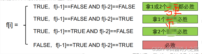
动态规划-硬币排成线
动态规划-硬币排成线 1 描述2 样例2.1 样例 1:2.2 样例 2:2.3 样例 3: 3 算法解题思路及实现3.1 算法解题分析3.1.1 确定状态3.1.2 转移方程3.1.3 初始条件和边界情况3.1.4 计算顺序 3.2 算法实现3.2.1 动态规划常规实现3.2.2 动态规划滚动数组 该题是lintcode的第394题&#x…...
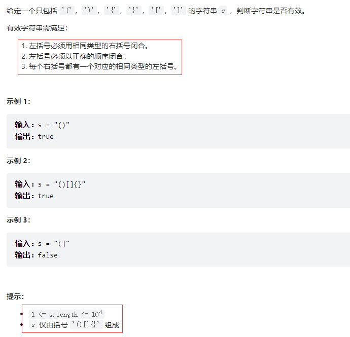
有效的括号——力扣20
题目描述 思路 1.判断括号的有效性可以使用「栈」这一数据结构来解决 2.遍历给定的字符串 s。当遇到一个左括号时,我们会期望在后续的遍历中,有一个相同类型的右括号将其闭合。由于后遇到的左括号要先闭合,因此我们可以将这个左括号放入栈顶。…...

【轻量级网络】华为诺亚:VanillaNet
文章目录 0. 前言1. 网络结构2. VanillaNet非线性表达能力增强策略2.1 深度训练2.2 扩展激活函数 3. 总结4. 参考 0. 前言 随着人工智能芯片的发展,神经网络推理速度的瓶颈不再是FLOPs或参数量,因为现代GPU可以很容易地进行计算能力较强的并行计算。相比…...
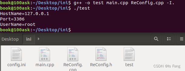
读写ini配置文件(C++)
文章目录 1、为什么要使用ini或者其它(例如xml,json)配置文件?2、ini文件基本介绍3、ini配置文件的格式4、C读写ini配置文件5、 代码示例6、 配置文件的解析库 文章转载于:https://blog.csdn.net/weixin_44517656/article/details/109014236 1、为什么要…...

Python对接亚马逊电商平台SP-API的一些概念理解准备
❝ 除了第三方服务商,其实亚马逊卖家本身也可以通过和SP-API的对接,利用程序来自动化亚马逊店铺销售运营管理中很多环节的工作,简单的应用比如可以利用SP-API的对接,实现亚马逊卖家后台各类报表的定期自动下载以及数据分析整理工…...

[Halcon3D] 主流的3D光学视觉方案及原理
📢博客主页:https://loewen.blog.csdn.net📢欢迎点赞 👍 收藏 ⭐留言 📝 如有错误敬请指正!📢本文由 丶布布原创,首发于 CSDN,转载注明出处🙉📢现…...

Go Web下gin框架使用(二)
〇、gin 路由 Gin是一个用于构建Web应用程序的Go语言框架,它具有简单、快速、灵活的特点。在Gin中,可以使用路由来定义URL和处理程序之间的映射关系。 r : gin.Default()// 访问 /index 这个路由// 获取信息r.GET("/index", func(c *gin.Con…...

算法笔记-线段树合并
线段树合并 前置知识:权值线段树、动态开点 将两棵线段树的信息合并成一棵线段树。 可以新建一颗线段树保存原来两颗线段树的信息,也可以将第二棵线段树维护的信息加到第一棵线段树上。 前者的空间复杂度较高,如果合并之前的线段树不会再用…...

Fiddler抓取IOS数据包实践教程
Fiddler是一个http协议调试代理工具,它能够记录并检查所有你的电脑和互联网之间的http通讯,设置断点,查看所有的“进出”Fiddler的数据(指cookie,html,js,css等文件)。 本章教程,主要介绍如何利用Fiddler抓取IOS数据包相关教程。 目录 一、打开Fiddler监听端口 二、配置网…...
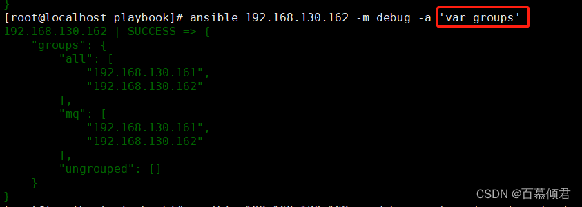
Ansible基础4——变量、机密、事实
文章目录 一、变量二、机密2.1 创建加密文件2.2 查看加密文件2.3 编辑加密文件内容2.4 加密现有文件2.5 解密文件2.6 更改加密密码 三、事实3.1 收集展示事实3.2 展示某个结果3.3 新旧事实命令3.4 关闭事实3.5 魔法变量 一、变量 常设置的变量: 要创建的用户要安装的…...

React实现Vue的watch监听属性
在 Vue 中可以简单地使用 watch 来监听数据的变化,还能获取到改变前的旧值,而在 React 中是没有 watch 的。 React中比较复杂,但是我们如果想在 React 中实现一个类似 Vue 的 watch 监听属性,也不是没有办法。 在React类组件中实…...

axios、跨域与JSONP、防抖和节流
文章目录 一、axios1、什么是axios2、axios发起GET请求3、axios发起POST请求4、直接使用axios发起请求 二、跨域与JSONP1、了解同源策略和跨域2、JSONP(1)实现一个简单的JSONP(2)JSONP的缺点(3)jQuery中的J…...

macOS Ventura 13.5beta2 (22G5038d)发布
系统介绍 黑果魏叔 6 月 1 日消息,苹果今日向 Mac 电脑用户推送了 macOS 13.5 开发者预览版 Beta 2 更新(内部版本号:22G5038d),本次更新距离上次发布隔了 12 天。 macOS Ventura 带来了台前调度、连续互通相机、Fac…...
jwt----介绍,原理
token:服务的生成的加密字符串,如果存在客户端浏览器上,就叫cookie -三部分:头,荷载,签名 -签发:登录成功,签发 -认证:认证类中认证 # jwt&…...

第19节 Node.js Express 框架
Express 是一个为Node.js设计的web开发框架,它基于nodejs平台。 Express 简介 Express是一个简洁而灵活的node.js Web应用框架, 提供了一系列强大特性帮助你创建各种Web应用,和丰富的HTTP工具。 使用Express可以快速地搭建一个完整功能的网站。 Expre…...
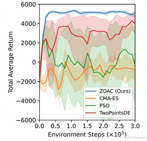
突破不可导策略的训练难题:零阶优化与强化学习的深度嵌合
强化学习(Reinforcement Learning, RL)是工业领域智能控制的重要方法。它的基本原理是将最优控制问题建模为马尔可夫决策过程,然后使用强化学习的Actor-Critic机制(中文译作“知行互动”机制),逐步迭代求解…...
练习(含atoi的模拟实现,自定义类型等练习)
一、结构体大小的计算及位段 (结构体大小计算及位段 详解请看:自定义类型:结构体进阶-CSDN博客) 1.在32位系统环境,编译选项为4字节对齐,那么sizeof(A)和sizeof(B)是多少? #pragma pack(4)st…...
cf2117E
原题链接:https://codeforces.com/contest/2117/problem/E 题目背景: 给定两个数组a,b,可以执行多次以下操作:选择 i (1 < i < n - 1),并设置 或,也可以在执行上述操作前执行一次删除任意 和 。求…...
select、poll、epoll 与 Reactor 模式
在高并发网络编程领域,高效处理大量连接和 I/O 事件是系统性能的关键。select、poll、epoll 作为 I/O 多路复用技术的代表,以及基于它们实现的 Reactor 模式,为开发者提供了强大的工具。本文将深入探讨这些技术的底层原理、优缺点。 一、I…...
tree 树组件大数据卡顿问题优化
问题背景 项目中有用到树组件用来做文件目录,但是由于这个树组件的节点越来越多,导致页面在滚动这个树组件的时候浏览器就很容易卡死。这种问题基本上都是因为dom节点太多,导致的浏览器卡顿,这里很明显就需要用到虚拟列表的技术&…...

云原生玩法三问:构建自定义开发环境
云原生玩法三问:构建自定义开发环境 引言 临时运维一个古董项目,无文档,无环境,无交接人,俗称三无。 运行设备的环境老,本地环境版本高,ssh不过去。正好最近对 腾讯出品的云原生 cnb 感兴趣&…...
提供了哪些便利?)
现有的 Redis 分布式锁库(如 Redisson)提供了哪些便利?
现有的 Redis 分布式锁库(如 Redisson)相比于开发者自己基于 Redis 命令(如 SETNX, EXPIRE, DEL)手动实现分布式锁,提供了巨大的便利性和健壮性。主要体现在以下几个方面: 原子性保证 (Atomicity)ÿ…...

Webpack性能优化:构建速度与体积优化策略
一、构建速度优化 1、升级Webpack和Node.js 优化效果:Webpack 4比Webpack 3构建时间降低60%-98%。原因: V8引擎优化(for of替代forEach、Map/Set替代Object)。默认使用更快的md4哈希算法。AST直接从Loa…...

根目录0xa0属性对应的Ntfs!_SCB中的FileObject是什么时候被建立的----NTFS源代码分析--重要
根目录0xa0属性对应的Ntfs!_SCB中的FileObject是什么时候被建立的 第一部分: 0: kd> g Breakpoint 9 hit Ntfs!ReadIndexBuffer: f7173886 55 push ebp 0: kd> kc # 00 Ntfs!ReadIndexBuffer 01 Ntfs!FindFirstIndexEntry 02 Ntfs!NtfsUpda…...