Kaggle(3):Predict CO2 Emissions in Rwanda
Kaggle(3):Predict CO2 Emissions in Rwanda

1. Introduction
在本次竞赛中,我们的任务是预测非洲 497 个不同地点 2022 年的二氧化碳排放量。 在训练数据中,我们有 2019-2021 年的二氧化碳排放量
本笔记本的内容:
1.通过平滑消除2020年一次性的新冠疫情趋势。 或者,用 2019 年和 2021 年的平均值来估算 2020 年也是一种有效的方法,但此处未实施
2. 观察靠近最大排放位置的位置也具有较高的排放水平。 执行 K-Means 聚类以根据数据点的位置对数据点进行聚类。 这允许具有相似排放的数据点被分组在一起
3. 以 2019 年和 2020 年为训练数据,用一些集成模型进行实验,以测试其在 2021 年数据上的 CV
import numpy as np
import pandas as pd
import matplotlib.pyplot as plt
import seaborn as sns
import math
from tqdm import tqdm
from sklearn.preprocessing import SplineTransformer
from holidays import CountryHoliday
from tqdm.notebook import tqdm
from typing import Listfrom category_encoders import OneHotEncoder, MEstimateEncoder, GLMMEncoder, OrdinalEncoder
from sklearn.model_selection import RepeatedStratifiedKFold, StratifiedKFold, KFold, RepeatedKFold, TimeSeriesSplit, train_test_split, cross_val_score
from sklearn.ensemble import ExtraTreesRegressor, RandomForestRegressor, GradientBoostingRegressor
from sklearn.ensemble import HistGradientBoostingRegressor, VotingRegressor, StackingRegressor
from sklearn.svm import SVR, LinearSVR
from sklearn.neighbors import KNeighborsRegressor
from sklearn.ensemble import RandomForestClassifier
from sklearn.linear_model import LinearRegression, Ridge, Lasso, ElasticNet, SGDRegressor, LogisticRegression
from sklearn.linear_model import PassiveAggressiveRegressor, ARDRegression
from sklearn.linear_model import TheilSenRegressor, RANSACRegressor, HuberRegressor
from sklearn.cross_decomposition import PLSRegression
from sklearn.neural_network import MLPRegressor
from sklearn.metrics import mean_squared_error, mean_absolute_error, roc_auc_score, roc_curve
from sklearn.metrics.pairwise import euclidean_distances
from sklearn.pipeline import Pipeline, make_pipeline
from sklearn.base import BaseEstimator, TransformerMixin
from sklearn.preprocessing import FunctionTransformer, StandardScaler, MinMaxScaler, LabelEncoder, SplineTransformer
from sklearn.compose import ColumnTransformer
from sklearn.impute import SimpleImputer, KNNImputer
from scipy.cluster.hierarchy import dendrogram, linkage
from scipy.spatial.distance import squareform
from sklearn.feature_selection import RFECV
from sklearn.decomposition import PCA
from xgboost import XGBRegressor, XGBClassifier
import lightgbm as lgbm
from lightgbm import LGBMRegressor, LGBMClassifier
from lightgbm import log_evaluation, early_stopping, record_evaluation
from catboost import CatBoostRegressor, CatBoostClassifier, Pool
from sklearn import set_config
from sklearn.multioutput import MultiOutputClassifier
from datetime import datetime, timedelta
import gcimport warnings
warnings.filterwarnings('ignore')set_config(transform_output = 'pandas')pal = sns.color_palette('viridis')pd.set_option('display.max_rows', 100)
M = 1.07
2. Examine Data
2.1
在这里,我们试图平滑 2020 年的数据以消除新冠趋势
1.使用平滑导入的数据集
2. 使用 2019 年和 2021 年值的平均值 [https://www.kaggle.com/code/kacperrabczewski/rwanda-co2-step-by-step-guide]
extrp = pd.read_csv("./data/PS3E20_train_covid_updated")
extrp = extrp[(extrp["year"] == 2020)]
extrp
| ID_LAT_LON_YEAR_WEEK | latitude | longitude | year | week_no | SulphurDioxide_SO2_column_number_density | SulphurDioxide_SO2_column_number_density_amf | SulphurDioxide_SO2_slant_column_number_density | SulphurDioxide_cloud_fraction | SulphurDioxide_sensor_azimuth_angle | ... | Cloud_cloud_top_height | Cloud_cloud_base_pressure | Cloud_cloud_base_height | Cloud_cloud_optical_depth | Cloud_surface_albedo | Cloud_sensor_azimuth_angle | Cloud_sensor_zenith_angle | Cloud_solar_azimuth_angle | Cloud_solar_zenith_angle | emission | |
|---|---|---|---|---|---|---|---|---|---|---|---|---|---|---|---|---|---|---|---|---|---|
| 53 | ID_-0.510_29.290_2020_00 | -0.510 | 29.290 | 2020 | 0 | 0.000064 | 0.970290 | 0.000073 | 0.163462 | -100.602665 | ... | 5388.602054 | 60747.063530 | 4638.602176 | 6.287709 | 0.283116 | -13.291375 | 33.679610 | -140.309173 | 30.053447 | 3.753601 |
| 54 | ID_-0.510_29.290_2020_01 | -0.510 | 29.290 | 2020 | 1 | NaN | NaN | NaN | NaN | NaN | ... | 6361.488754 | 53750.174162 | 5361.488754 | 19.167269 | 0.317732 | -30.474972 | 48.119754 | -139.437777 | 30.391957 | 4.051966 |
| 55 | ID_-0.510_29.290_2020_02 | -0.510 | 29.290 | 2020 | 2 | -0.000361 | 0.668526 | -0.000231 | 0.086199 | 73.269733 | ... | 5320.715902 | 61012.625000 | 4320.715861 | 48.203733 | 0.265554 | -12.461150 | 35.809728 | -137.854449 | 29.100415 | 4.154116 |
| 56 | ID_-0.510_29.290_2020_03 | -0.510 | 29.290 | 2020 | 3 | 0.000597 | 0.553729 | 0.000331 | 0.149257 | 73.522247 | ... | 6219.319294 | 55704.782998 | 5219.319269 | 12.809350 | 0.267030 | 16.381079 | 35.836898 | -139.017754 | 26.265561 | 4.165751 |
| 57 | ID_-0.510_29.290_2020_04 | -0.510 | 29.290 | 2020 | 4 | 0.000107 | 1.045238 | 0.000112 | 0.224283 | 77.588455 | ... | 6348.560006 | 54829.331776 | 5348.560014 | 35.283981 | 0.268983 | -12.193650 | 47.092968 | -134.474279 | 27.061321 | 4.233635 |
| ... | ... | ... | ... | ... | ... | ... | ... | ... | ... | ... | ... | ... | ... | ... | ... | ... | ... | ... | ... | ... | ... |
| 78965 | ID_-3.299_30.301_2020_48 | -3.299 | 30.301 | 2020 | 48 | 0.000114 | 1.123935 | 0.000125 | 0.149885 | 74.376836 | ... | 6092.323722 | 57479.397776 | 5169.185142 | 15.331296 | 0.261608 | 16.309625 | 39.924967 | -132.258700 | 30.393604 | 26.929207 |
| 78966 | ID_-3.299_30.301_2020_49 | -3.299 | 30.301 | 2020 | 49 | 0.000051 | 0.617927 | 0.000031 | 0.213135 | 72.364738 | ... | 5992.053006 | 57739.300155 | 4992.053006 | 27.214085 | 0.276616 | -0.287656 | 45.624810 | -134.460418 | 30.911741 | 26.606790 |
| 78967 | ID_-3.299_30.301_2020_50 | -3.299 | 30.301 | 2020 | 50 | -0.000235 | 0.633192 | -0.000149 | 0.257000 | -99.141518 | ... | 6104.231241 | 56954.517231 | 5181.570213 | 26.270365 | 0.260574 | -50.411241 | 37.645974 | -132.193161 | 32.516685 | 27.256273 |
| 78968 | ID_-3.299_30.301_2020_51 | -3.299 | 30.301 | 2020 | 51 | NaN | NaN | NaN | NaN | NaN | ... | 4855.537585 | 64839.955718 | 3858.187453 | 14.519789 | 0.248484 | 30.840922 | 39.529722 | -138.964016 | 28.574091 | 25.591976 |
| 78969 | ID_-3.299_30.301_2020_52 | -3.299 | 30.301 | 2020 | 52 | 0.000025 | 1.103025 | 0.000028 | 0.265622 | -99.811790 | ... | 5345.679464 | 62098.716546 | 4345.679397 | 13.082162 | 0.283677 | -13.002957 | 38.243055 | -136.660958 | 29.584058 | 25.559870 |
26341 rows × 76 columns
DATA_DIR = "./data/"
train = pd.read_csv(DATA_DIR + "train.csv")
test = pd.read_csv(DATA_DIR + "test.csv")def add_features(df):#df["week"] = df["year"].astype(str) + "-" + df["week_no"].astype(str)#df["date"] = df["week"].apply(lambda x: get_date_from_week_string(x))#df = df.drop(columns = ["week"])df["week"] = (df["year"] - 2019) * 53 + df["week_no"]#df["lat_long"] = df["latitude"].astype(str) + "#" + df["longitude"].astype(str)return dftrain = add_features(train)
test = add_features(test)
2.2
对预测进行一些有风险的后处理。
假设数据点的 MAX = max(2019 年排放量、2020 年排放量、2021 年排放量)。
如果 2021 年排放量 > 2019 年排放量,我们将 MAX * 1.07 分配给预测,否则我们只分配 MAX。 参考:https://www.kaggle.com/competitions/playground-series-s3e20/discussion/430152
vals = set()
for x in train[["latitude", "longitude"]].values:vals.add(tuple(x))vals = list(vals)
zeros = []for lat, long in vals:subset = train[(train["latitude"] == lat) & (train["longitude"] == long)]em_vals = subset["emission"].valuesif all(x == 0 for x in em_vals):zeros.append([lat, long])
test["2021_emission"] = test["week_no"]
test["2020_emission"] = test["week_no"]
test["2019_emission"] = test["week_no"]for lat, long in vals:test.loc[(test.latitude == lat) & (test.longitude == long), "2021_emission"] = train.loc[(train.latitude == lat) & (train.longitude == long) & (train.year == 2021) & (train.week_no <= 48), "emission"].valuestest.loc[(test.latitude == lat) & (test.longitude == long), "2020_emission"] = train.loc[(train.latitude == lat) & (train.longitude == long) & (train.year == 2020) & (train.week_no <= 48), "emission"].valuestest.loc[(test.latitude == lat) & (test.longitude == long), "2019_emission"] = train.loc[(train.latitude == lat) & (train.longitude == long) & (train.year == 2019) & (train.week_no <= 48), "emission"].values#print(train.loc[(train.latitude == lat) & (train.longitude == long) & (train.year == 2021), "emission"])test["ratio"] = (test["2021_emission"] / test["2019_emission"]).replace(np.nan, 0)
test["pos_ratio"] = test["ratio"].apply(lambda x: max(x, 1))
test["pos_ratio"] = test["pos_ratio"].apply(lambda x: 1.07 if x > 1 else x)
test["max"] = test[["2019_emission", "2020_emission", "2021_emission"]].max(axis=1)
test["lazy_pred"] = test["max"] * test["pos_ratio"]
test = test.drop(columns = ["ratio", "pos_ratio", "max", "2019_emission", "2020_emission", "2021_emission"])
train.loc[train.year == 2020, "emission"] = extrp
train
| ID_LAT_LON_YEAR_WEEK | latitude | longitude | year | week_no | SulphurDioxide_SO2_column_number_density | SulphurDioxide_SO2_column_number_density_amf | SulphurDioxide_SO2_slant_column_number_density | SulphurDioxide_cloud_fraction | SulphurDioxide_sensor_azimuth_angle | ... | Cloud_cloud_base_pressure | Cloud_cloud_base_height | Cloud_cloud_optical_depth | Cloud_surface_albedo | Cloud_sensor_azimuth_angle | Cloud_sensor_zenith_angle | Cloud_solar_azimuth_angle | Cloud_solar_zenith_angle | emission | week | |
|---|---|---|---|---|---|---|---|---|---|---|---|---|---|---|---|---|---|---|---|---|---|
| 0 | ID_-0.510_29.290_2019_00 | -0.510 | 29.290 | 2019 | 0 | -0.000108 | 0.603019 | -0.000065 | 0.255668 | -98.593887 | ... | 61085.809570 | 2615.120483 | 15.568533 | 0.272292 | -12.628986 | 35.632416 | -138.786423 | 30.752140 | 3.750994 | 0 |
| 1 | ID_-0.510_29.290_2019_01 | -0.510 | 29.290 | 2019 | 1 | 0.000021 | 0.728214 | 0.000014 | 0.130988 | 16.592861 | ... | 66969.478735 | 3174.572424 | 8.690601 | 0.256830 | 30.359375 | 39.557633 | -145.183930 | 27.251779 | 4.025176 | 1 |
| 2 | ID_-0.510_29.290_2019_02 | -0.510 | 29.290 | 2019 | 2 | 0.000514 | 0.748199 | 0.000385 | 0.110018 | 72.795837 | ... | 60068.894448 | 3516.282669 | 21.103410 | 0.251101 | 15.377883 | 30.401823 | -142.519545 | 26.193296 | 4.231381 | 2 |
| 3 | ID_-0.510_29.290_2019_03 | -0.510 | 29.290 | 2019 | 3 | NaN | NaN | NaN | NaN | NaN | ... | 51064.547339 | 4180.973322 | 15.386899 | 0.262043 | -11.293399 | 24.380357 | -132.665828 | 28.829155 | 4.305286 | 3 |
| 4 | ID_-0.510_29.290_2019_04 | -0.510 | 29.290 | 2019 | 4 | -0.000079 | 0.676296 | -0.000048 | 0.121164 | 4.121269 | ... | 63751.125781 | 3355.710107 | 8.114694 | 0.235847 | 38.532263 | 37.392979 | -141.509805 | 22.204612 | 4.347317 | 4 |
| ... | ... | ... | ... | ... | ... | ... | ... | ... | ... | ... | ... | ... | ... | ... | ... | ... | ... | ... | ... | ... | ... |
| 79018 | ID_-3.299_30.301_2021_48 | -3.299 | 30.301 | 2021 | 48 | 0.000284 | 1.195643 | 0.000340 | 0.191313 | 72.820518 | ... | 60657.101913 | 4590.879504 | 20.245954 | 0.304797 | -35.140368 | 40.113533 | -129.935508 | 32.095214 | 29.404171 | 154 |
| 79019 | ID_-3.299_30.301_2021_49 | -3.299 | 30.301 | 2021 | 49 | 0.000083 | 1.130868 | 0.000063 | 0.177222 | -12.856753 | ... | 60168.191528 | 4659.130378 | 6.104610 | 0.314015 | 4.667058 | 47.528435 | -134.252871 | 30.771469 | 29.186497 | 155 |
| 79020 | ID_-3.299_30.301_2021_50 | -3.299 | 30.301 | 2021 | 50 | NaN | NaN | NaN | NaN | NaN | ... | 56596.027209 | 5222.646823 | 14.817885 | 0.288058 | -0.340922 | 35.328098 | -134.731723 | 30.716166 | 29.131205 | 156 |
| 79021 | ID_-3.299_30.301_2021_51 | -3.299 | 30.301 | 2021 | 51 | -0.000034 | 0.879397 | -0.000028 | 0.184209 | -100.344827 | ... | 46533.348194 | 6946.858022 | 32.594768 | 0.274047 | 8.427699 | 48.295652 | -139.447849 | 29.112868 | 28.125792 | 157 |
| 79022 | ID_-3.299_30.301_2021_52 | -3.299 | 30.301 | 2021 | 52 | -0.000091 | 0.871951 | -0.000079 | 0.000000 | 76.825638 | ... | 47771.681887 | 6553.295018 | 19.464032 | 0.226276 | -12.808528 | 47.923441 | -136.299984 | 30.246387 | 27.239302 | 158 |
79023 rows × 77 columns
test
| ID_LAT_LON_YEAR_WEEK | latitude | longitude | year | week_no | SulphurDioxide_SO2_column_number_density | SulphurDioxide_SO2_column_number_density_amf | SulphurDioxide_SO2_slant_column_number_density | SulphurDioxide_cloud_fraction | SulphurDioxide_sensor_azimuth_angle | ... | Cloud_cloud_base_pressure | Cloud_cloud_base_height | Cloud_cloud_optical_depth | Cloud_surface_albedo | Cloud_sensor_azimuth_angle | Cloud_sensor_zenith_angle | Cloud_solar_azimuth_angle | Cloud_solar_zenith_angle | week | lazy_pred | |
|---|---|---|---|---|---|---|---|---|---|---|---|---|---|---|---|---|---|---|---|---|---|
| 0 | ID_-0.510_29.290_2022_00 | -0.510 | 29.290 | 2022 | 0 | NaN | NaN | NaN | NaN | NaN | ... | 41047.937500 | 7472.313477 | 7.935617 | 0.240773 | -100.113792 | 33.697044 | -133.047546 | 33.779583 | 159 | 3.753601 |
| 1 | ID_-0.510_29.290_2022_01 | -0.510 | 29.290 | 2022 | 1 | 0.000456 | 0.691164 | 0.000316 | 0.000000 | 76.239196 | ... | 54915.708579 | 5476.147161 | 11.448437 | 0.293119 | -30.510319 | 42.402593 | -138.632822 | 31.012380 | 160 | 4.051966 |
| 2 | ID_-0.510_29.290_2022_02 | -0.510 | 29.290 | 2022 | 2 | 0.000161 | 0.605107 | 0.000106 | 0.079870 | -42.055341 | ... | 39006.093750 | 7984.795703 | 10.753179 | 0.267130 | 39.087361 | 45.936480 | -144.784988 | 26.743361 | 161 | 4.231381 |
| 3 | ID_-0.510_29.290_2022_03 | -0.510 | 29.290 | 2022 | 3 | 0.000350 | 0.696917 | 0.000243 | 0.201028 | 72.169566 | ... | 57646.368368 | 5014.724115 | 11.764556 | 0.304679 | -24.465127 | 42.140419 | -135.027891 | 29.604774 | 162 | 4.305286 |
| 4 | ID_-0.510_29.290_2022_04 | -0.510 | 29.290 | 2022 | 4 | -0.000317 | 0.580527 | -0.000184 | 0.204352 | 76.190865 | ... | 52896.541873 | 5849.280394 | 13.065317 | 0.284221 | -12.907850 | 30.122641 | -135.500119 | 26.276807 | 163 | 4.347317 |
| ... | ... | ... | ... | ... | ... | ... | ... | ... | ... | ... | ... | ... | ... | ... | ... | ... | ... | ... | ... | ... | ... |
| 24348 | ID_-3.299_30.301_2022_44 | -3.299 | 30.301 | 2022 | 44 | -0.000618 | 0.745549 | -0.000461 | 0.234492 | 72.306198 | ... | 55483.459980 | 5260.120056 | 30.398508 | 0.180046 | -25.528588 | 45.284576 | -116.521412 | 29.992562 | 203 | 30.327420 |
| 24349 | ID_-3.299_30.301_2022_45 | -3.299 | 30.301 | 2022 | 45 | NaN | NaN | NaN | NaN | NaN | ... | 53589.917383 | 5678.951521 | 19.223844 | 0.177833 | -13.380005 | 43.770351 | -122.405759 | 29.017975 | 204 | 30.811167 |
| 24350 | ID_-3.299_30.301_2022_46 | -3.299 | 30.301 | 2022 | 46 | NaN | NaN | NaN | NaN | NaN | ... | 62646.761340 | 4336.282491 | 13.801194 | 0.219471 | -5.072065 | 33.226455 | -124.530639 | 30.187472 | 205 | 31.162886 |
| 24351 | ID_-3.299_30.301_2022_47 | -3.299 | 30.301 | 2022 | 47 | 0.000071 | 1.003805 | 0.000077 | 0.205077 | 74.327427 | ... | 50728.313991 | 6188.578464 | 27.887489 | 0.247275 | -0.668714 | 45.885617 | -129.006797 | 30.427455 | 206 | 31.439606 |
| 24352 | ID_-3.299_30.301_2022_48 | -3.299 | 30.301 | 2022 | 48 | NaN | NaN | NaN | NaN | NaN | ... | 46260.039092 | 6777.863819 | 23.771269 | 0.239684 | -40.826139 | 30.680056 | -124.895473 | 34.457720 | 207 | 29.944366 |
24353 rows × 77 columns
Insights
训练数据集有 79023 个观测值,测试数据集有 24353 个观测值。 正如我们所观察到的,某些列具有空值
3. EDA and Data Distribution
def plot_emission(train):plt.figure(figsize=(15, 6))sns.lineplot(data=train, x="week", y="emission", label="Emission", alpha=0.7, color='blue')plt.xlabel('Week')plt.ylabel('Emission')plt.title('Emission over time')plt.legend()plt.tight_layout()plt.show()plot_emission(train)

sns.histplot(train["emission"])
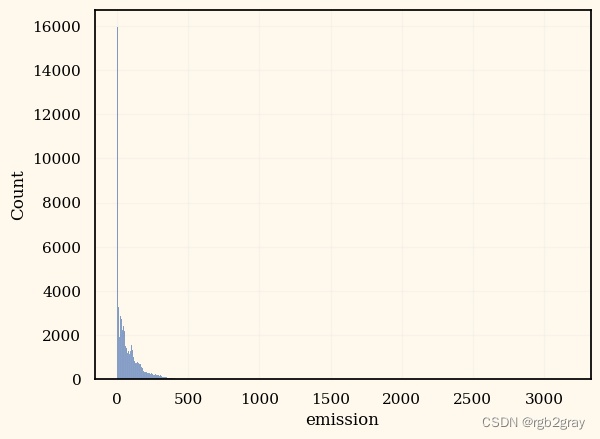
4. Data Transformation
print(len(vals))
497
Insights
有 497 个独特的经纬度组合
4.1
大多数特征只是噪音,我们可以将它们删除。(Reference: multiple discussion posts)
#train = train.drop(columns = ["ID_LAT_LON_YEAR_WEEK", "lat_long"])
#test = test.drop(columns = ["ID_LAT_LON_YEAR_WEEK", "lat_long"])train = train[["latitude", "longitude", "year", "week_no", "emission"]]
test = test[["latitude", "longitude", "year", "week_no", "lazy_pred"]]
4.2
K Means 聚类 + 到最高排放量的距离
#https://www.kaggle.com/code/lucasboesen/simple-catboost-6-features-cv-21-7
from sklearn.cluster import KMeans
import haversine as hskm_train = train.groupby(by=['latitude', 'longitude'], as_index=False)['emission'].mean()
model = KMeans(n_clusters = 7, random_state = 42)
model.fit(km_train)
yhat_train = model.predict(km_train)
km_train['kmeans_group'] = yhat_train""" Own Groups """
# Some locations have emission == 0
km_train['is_zero'] = km_train['emission'].apply(lambda x: 'no_emission_recorded' if x==0 else 'emission_recorded')# Distance to the highest emission location
max_lat_lon_emission = km_train.loc[km_train['emission']==km_train['emission'].max(), ['latitude', 'longitude']]
km_train['distance_to_max_emission'] = km_train.apply(lambda x: hs.haversine((x['latitude'], x['longitude']), (max_lat_lon_emission['latitude'].values[0], max_lat_lon_emission['longitude'].values[0])), axis=1)train = train.merge(km_train[['latitude', 'longitude', 'kmeans_group', 'distance_to_max_emission']], on=['latitude', 'longitude'])
test = test.merge(km_train[['latitude', 'longitude', 'kmeans_group', 'distance_to_max_emission']], on=['latitude', 'longitude'])
#train = train.drop(columns = ["latitude", "longitude"])
#test = test.drop(columns = ["latitude", "longitude"])
train
| latitude | longitude | year | week_no | emission | kmeans_group | distance_to_max_emission | |
|---|---|---|---|---|---|---|---|
| 0 | -0.510 | 29.290 | 2019 | 0 | 3.750994 | 6 | 207.849890 |
| 1 | -0.510 | 29.290 | 2019 | 1 | 4.025176 | 6 | 207.849890 |
| 2 | -0.510 | 29.290 | 2019 | 2 | 4.231381 | 6 | 207.849890 |
| 3 | -0.510 | 29.290 | 2019 | 3 | 4.305286 | 6 | 207.849890 |
| 4 | -0.510 | 29.290 | 2019 | 4 | 4.347317 | 6 | 207.849890 |
| ... | ... | ... | ... | ... | ... | ... | ... |
| 79018 | -3.299 | 30.301 | 2021 | 48 | 29.404171 | 6 | 157.630611 |
| 79019 | -3.299 | 30.301 | 2021 | 49 | 29.186497 | 6 | 157.630611 |
| 79020 | -3.299 | 30.301 | 2021 | 50 | 29.131205 | 6 | 157.630611 |
| 79021 | -3.299 | 30.301 | 2021 | 51 | 28.125792 | 6 | 157.630611 |
| 79022 | -3.299 | 30.301 | 2021 | 52 | 27.239302 | 6 | 157.630611 |
79023 rows × 7 columns
test
| latitude | longitude | year | week_no | lazy_pred | kmeans_group | distance_to_max_emission | |
|---|---|---|---|---|---|---|---|
| 0 | -0.510 | 29.290 | 2022 | 0 | 3.753601 | 6 | 207.849890 |
| 1 | -0.510 | 29.290 | 2022 | 1 | 4.051966 | 6 | 207.849890 |
| 2 | -0.510 | 29.290 | 2022 | 2 | 4.231381 | 6 | 207.849890 |
| 3 | -0.510 | 29.290 | 2022 | 3 | 4.305286 | 6 | 207.849890 |
| 4 | -0.510 | 29.290 | 2022 | 4 | 4.347317 | 6 | 207.849890 |
| ... | ... | ... | ... | ... | ... | ... | ... |
| 24348 | -3.299 | 30.301 | 2022 | 44 | 30.327420 | 6 | 157.630611 |
| 24349 | -3.299 | 30.301 | 2022 | 45 | 30.811167 | 6 | 157.630611 |
| 24350 | -3.299 | 30.301 | 2022 | 46 | 31.162886 | 6 | 157.630611 |
| 24351 | -3.299 | 30.301 | 2022 | 47 | 31.439606 | 6 | 157.630611 |
| 24352 | -3.299 | 30.301 | 2022 | 48 | 29.944366 | 6 | 157.630611 |
24353 rows × 7 columns
cat_params = {'n_estimators': 799, 'learning_rate': 0.09180872710592884,'depth': 8, 'l2_leaf_reg': 1.0242996861886846, 'subsample': 0.38227256755249117, 'colsample_bylevel': 0.7183481537623551,'random_state': 42,"silent": True,
}lgb_params = {'n_estimators': 835, 'max_depth': 12, 'reg_alpha': 3.849279869880706, 'reg_lambda': 0.6840221712299135, 'min_child_samples': 10, 'subsample': 0.6810493885301987, 'learning_rate': 0.0916362259866008, 'colsample_bytree': 0.3133780298325982, 'colsample_bynode': 0.7966712089198238,"random_state": 42,
}xgb_params = {"random_state": 42,
}rf_params = {'n_estimators': 263, 'max_depth': 41, 'min_samples_split': 10, 'min_samples_leaf': 3,"random_state": 42,"verbose": 0
}et_params = {"random_state": 42,"verbose": 0
}
5. Validate Performance on 2021 data
def rmse(a, b):return mean_squared_error(a, b, squared=False)
validation = train[train.year == 2021]
clusters = train["kmeans_group"].unique()for i in range(len(clusters)):cluster = clusters[i]print("==============================================")print(f" Cluster {cluster} ")train_c = train[train["kmeans_group"] == cluster]X_train = train_c[train_c.year < 2021].drop(columns = ["emission", "kmeans_group"])y_train = train_c[train_c.year < 2021]["emission"].copy()X_val = train_c[train_c.year >= 2021].drop(columns = ["emission", "kmeans_group"])y_val = train_c[train_c.year >= 2021]["emission"].copy()#=======================================================================================catboost_reg = CatBoostRegressor(**cat_params)catboost_reg.fit(X_train, y_train, eval_set=(X_val, y_val))catboost_pred = catboost_reg.predict(X_val) * Mprint(f"RMSE of CatBoost: {rmse(catboost_pred, y_val)}")#=======================================================================================lightgbm_reg = LGBMRegressor(**lgb_params,verbose=-1)lightgbm_reg.fit(X_train, y_train, eval_set=(X_val, y_val))lightgbm_pred = lightgbm_reg.predict(X_val) * Mprint(f"RMSE of LightGBM: {rmse(lightgbm_pred, y_val)}")#=======================================================================================xgb_reg = XGBRegressor(**xgb_params)xgb_reg.fit(X_train, y_train, eval_set=[(X_val, y_val)], verbose = False)xgb_pred = xgb_reg.predict(X_val) * Mprint(f"RMSE of XGBoost: {rmse(xgb_pred, y_val)}")#=======================================================================================rf_reg = RandomForestRegressor(**rf_params)rf_reg.fit(X_train, y_train)rf_pred = rf_reg.predict(X_val) * Mprint(f"RMSE of Random Forest: {rmse(rf_pred, y_val)}")#=======================================================================================et_reg = ExtraTreesRegressor(**et_params)et_reg.fit(X_train, y_train)et_pred = et_reg.predict(X_val) * Mprint(f"RMSE of Extra Trees: {rmse(et_pred, y_val)}")overall_pred = lightgbm_pred #(catboost_pred + lightgbm_pred) / 2validation.loc[validation["kmeans_group"] == cluster, "emission"] = overall_predprint(f"RMSE Overall: {rmse(overall_pred, y_val)}")print("==============================================")
print(f"[DONE] RMSE of all clusters: {rmse(validation['emission'], train[train.year == 2021]['emission'])}")
print(f"[DONE] RMSE of all clusters Week 1-20: {rmse(validation[validation.week_no < 21]['emission'], train[(train.year == 2021) & (train.week_no < 21)]['emission'])}")
print(f"[DONE] RMSE of all clusters Week 21+: {rmse(validation[validation.week_no >= 21]['emission'], train[(train.year == 2021) & (train.week_no  >= 21)]['emission'])}")
==============================================Cluster 6
RMSE of CatBoost: 2.3575606902299895
RMSE of LightGBM: 2.2103640167714094
RMSE of XGBoost: 2.5018849673349863
RMSE of Random Forest: 2.6335510523545556
RMSE of Extra Trees: 3.0029623116826776
RMSE Overall: 2.2103640167714094
==============================================Cluster 5
RMSE of CatBoost: 19.175306730779514
RMSE of LightGBM: 17.910821889134688
RMSE of XGBoost: 19.6677120674706
RMSE of Random Forest: 18.856743714624777
RMSE of Extra Trees: 20.70417439300032
RMSE Overall: 17.910821889134688
==============================================Cluster 1
RMSE of CatBoost: 9.26195004601851
RMSE of LightGBM: 8.513309514506675
RMSE of XGBoost: 10.137965612920658
RMSE of Random Forest: 9.838001199034126
RMSE of Extra Trees: 11.043246766709913
RMSE Overall: 8.513309514506675
==============================================Cluster 4
RMSE of CatBoost: 44.564695183442716
RMSE of LightGBM: 43.946690922308754
RMSE of XGBoost: 50.18811358270916
RMSE of Random Forest: 46.39201148051631
RMSE of Extra Trees: 50.58999576441371
RMSE Overall: 43.946690922308754
==============================================Cluster 0
RMSE of CatBoost: 28.408461784012662
RMSE of LightGBM: 26.872533954605416
RMSE of XGBoost: 30.622689084145943
RMSE of Random Forest: 28.46657485784377
RMSE of Extra Trees: 31.733046766544884
RMSE Overall: 26.872533954605416
==============================================Cluster 3
RMSE of CatBoost: 263.29528869714665
RMSE of LightGBM: 326.12883397111284
RMSE of XGBoost: 336.5771065570381
RMSE of Random Forest: 303.9321016178147
RMSE of Extra Trees: 336.67756932119914
RMSE Overall: 326.12883397111284
==============================================Cluster 2
RMSE of CatBoost: 206.96165808156715
RMSE of LightGBM: 222.40891682146665
RMSE of XGBoost: 281.12604107718465
RMSE of Random Forest: 232.11332438348992
RMSE of Extra Trees: 281.29392713471816
RMSE Overall: 222.40891682146665
==============================================
[DONE] RMSE of all clusters: 23.275548123498453
[DONE] RMSE of all clusters Week 1-20: 31.92891146501802
[DONE] RMSE of all clusters Week 21+: 15.108200701163458
6. Predicting 2022 result
clusters = train["kmeans_group"].unique()for i in tqdm(range(len(clusters))):cluster = clusters[i]train_c = train[train["kmeans_group"] == cluster]if "emission" in test.columns:test_c = test[test["kmeans_group"] == cluster].drop(columns = ["emission", "kmeans_group", "lazy_pred"])else:test_c = test[test["kmeans_group"] == cluster].drop(columns = ["kmeans_group", "lazy_pred"])X = train_c.drop(columns = ["emission", "kmeans_group"])y = train_c["emission"].copy()#=======================================================================================catboost_reg = CatBoostRegressor(**cat_params)catboost_reg.fit(X, y)#print(test_c)catboost_pred = catboost_reg.predict(test_c)#=======================================================================================lightgbm_reg = LGBMRegressor(**lgb_params,verbose=-1)lightgbm_reg.fit(X, y)#print(test_c)lightgbm_pred = lightgbm_reg.predict(test_c)#=======================================================================================#xgb_reg = XGBRegressor(**xgb_params)#xgb_reg.fit(X, y, verbose = False)#xgb_pred = xgb_reg.predict(test)#=======================================================================================rf_reg = RandomForestRegressor(**rf_params)rf_reg.fit(X, y)rf_pred = rf_reg.predict(test_c)#=======================================================================================#et_reg = ExtraTreesRegressor(**et_params)#et_reg.fit(X, y)#et_pred = et_reg.predict(test)overall_pred = lightgbm_pred #(catboost_pred + lightgbm_pred) / 2test.loc[test["kmeans_group"] == cluster, "emission"] = overall_pred
0%| | 0/7 [00:00<?, ?it/s]
test["emission"] = test["emission"] * 1.07
test.to_csv('submission.csv', index=False)
相关文章:
Kaggle(3):Predict CO2 Emissions in Rwanda
Kaggle(3):Predict CO2 Emissions in Rwanda 1. Introduction 在本次竞赛中,我们的任务是预测非洲 497 个不同地点 2022 年的二氧化碳排放量。 在训练数据中,我们有 2019-2021 年的二氧化碳排放量 本笔记本的内容&am…...

【技巧分享】如何获取子窗体选择了多少记录数?一招搞定!
Hi,大家好久不见。 我这个更新速度是不是太慢了呀,因为,最近又又又在忙,请大家谅解啦。 现在更新文章、视频都要花好久去考虑,好不容易有个灵感了,一搜索,结果发现之前都已经分享过了(委屈脸&…...

Kotlin AQ
如何学习kotlin? 学习Kotlin的步骤如下: 1. 理解Kotlin的基础:首先,你需要理解Kotlin的基础知识,包括变量、数据类型、运算符、控制流等。你可以通过阅读Kotlin的官方文档或者其他在线教程来学习。 2. 实践编程:理论…...
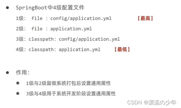
SpringBoot入门篇2 - 配置文件格式、多环境开发、配置文件分类
目录 1.配置文件格式(3种) 例:修改服务器端口。(3种) src/main/resources/application.properties server.port80 src/main/resources/application.yml(主要用这种) server:port: 80 src/m…...

UOS安装6.1.11内核或4.19内核
6.1.11内核 sudo sh -c echo "deb https://proposed-packages.deepin.com/beige-testing unstable main dde community commercial " > /etc/apt/sources.list.d/deepin-testing.list sudo apt update && sudo apt install linux-image-6.1.11-amd64-de…...

HiveSQL刷题
41、同时在线人数问题 现有各直播间的用户访问记录表(live_events)如下,表中每行数据表达的信息为,一个用户何时进入了一个直播间,又在何时离开了该直播间。 user_id (用户id)live_id (直播间id)in_datetime (进入直…...

path路径模块
path模块是Node.js官方提供的、用来处理路径的模块。它提供了一系列的方法和属性,用来满足用户对路径的处理需求。 path.join( )用来将多个路径片段拼接成一个完整的路径字符串 ../会抵消前面的路径 const path require(path) const pathStr path.join(/a,/b,../,/d) conso…...
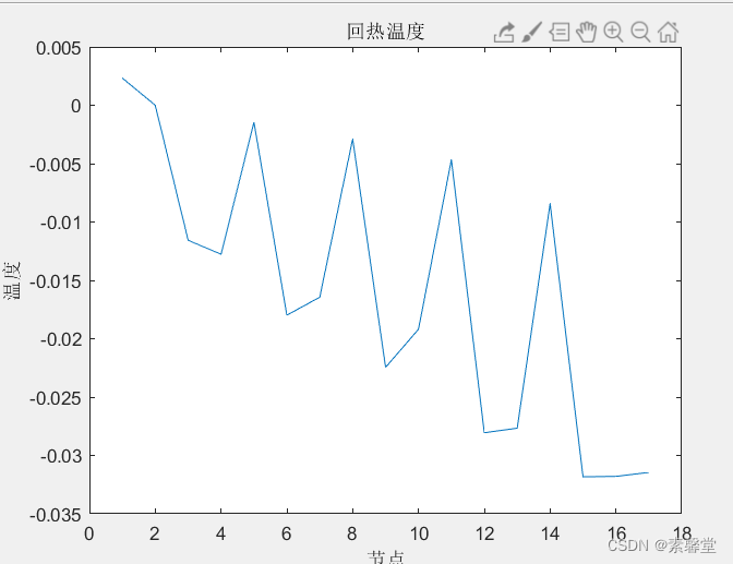
1.文章复现《热电联产系统在区域综合能源系统中的定容选址研究》(附matlab程序)
0.代码链接 文章复现《热电联产系统在区域综合能源系统中的定容选址研究》(matlab程序)-Matlab文档类资源-CSDN文库 1.简述 本文采用遗传算法的方式进行了下述文章的复现并采用电-热节点的方式进行了潮流计算以降低电网的网络损耗 分析了电网的基本数…...
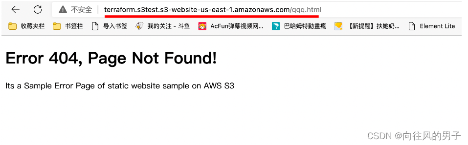
【Terraform学习】使用 Terraform 托管 S3 静态网站(Terraform-AWS最佳实战学习)
使用 Terraform 托管 S3 静态网站 实验步骤 前提条件 安装 Terraform: 地址 下载仓库代码模版 本实验代码位于 task_s3 文件夹中。 变量文件 variables.tf 在上面的代码中,您将声明,aws_access_key,aws_secret_key和区域变量…...

触发JVM fatal error并配置相关JVM参数
1. 絮絮叨叨 工作中,Java服务因为fatal error(致命错误,笔者称其为jvm crash),在服务运行日志中出现了致命错误的概要信息: # # A fatal error has been detected by the Java Runtime Environment: # # S…...
爬虫(bilibili热门课程记录)
什么是爬虫?程序蜘蛛,沿着互联网获取相关信息,收集目标信息。 一、python环境安装 1、先从Download Python | Python.org中下载最新版本的python解释器 2、再从Download PyCharm: Python IDE for Professional Developers by JetBrains中下…...
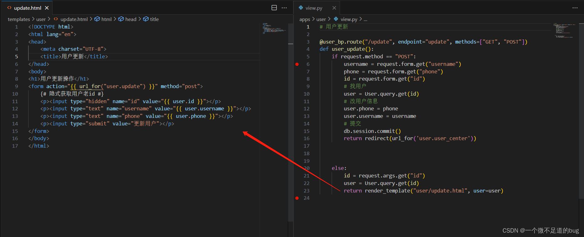
14-模型 - 增删改查
增: # 1. 找到模型类并创建对象 user User() # 2. 给对象的属性赋值 user.username username user.password password user.phone phone # 3. 将user对象添加到session中 (类似缓存) db.session.add(user) # 4. 提交数据 db.session.commit() 删: # 两种删除:# 1. 逻辑删…...

C#与西门子PLC1500的ModbusTcp服务器通信3--搭建ModbusTcp服务器
1、打开仿真工具,创建PLC,注意创建完成后不要关闭 注意,这个IP地址必须与西门子虚拟网卡的IP地址及虚拟机的网卡IP地址同一网段 2、打开博途V15,创建项目,命名为Lan项目 3、添加1500系列CPU1513 4、设置设置IP地址及属…...
Linux系统编程:线程控制
目录 一. 线程的创建 1.1 pthread_create函数 1.2 线程id的本质 二. 多线程中的异常和程序替换 2.1 多线程程序异常 2.2 多线程中的程序替换 三. 线程等待 四. 线程的终止和分离 4.1 线程函数return 4.2 线程取消 pthread_cancel 4.3 线程退出 pthread_exit 4.4 线程…...

基于Java+SpringBoot+Vue前后端分离纺织品企业财务管理系统设计和实现
博主介绍:✌全网粉丝30W,csdn特邀作者、博客专家、CSDN新星计划导师、Java领域优质创作者,博客之星、掘金/华为云/阿里云/InfoQ等平台优质作者、专注于Java技术领域和毕业项目实战✌ 🍅文末获取源码联系🍅 👇🏻 精彩专…...

搭建开发环境-Windows
写C# 的请出去。 然后,Windows 是最好的Linux发行版。搭建开发环境-WSLUbuntu...
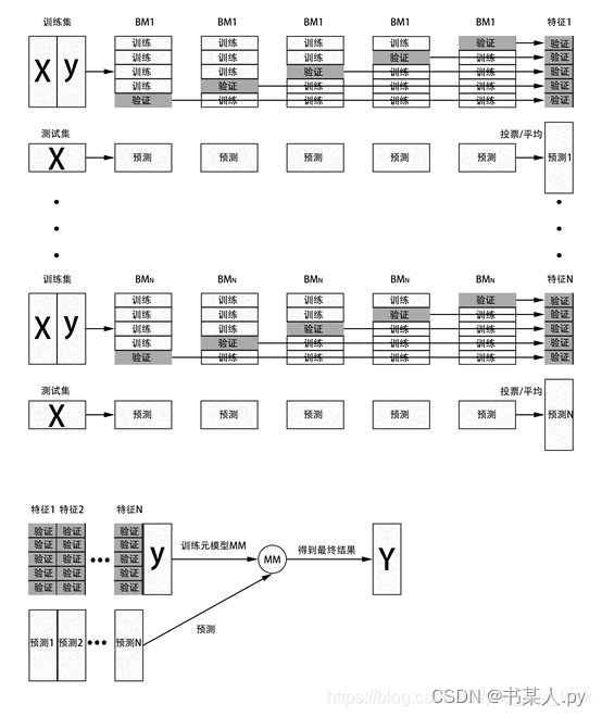
【 Python 全栈开发 - 人工智能篇 - 45 】集成算法与聚类算法
文章目录 一、集成算法1.1 概念1.2 常用集成算法1.2.1 Bagging1.2.2 Boosting1.2.2.1 AdaBoost1.2.2.2 GBDT1.2.2.3 XgBoost 1.2.3 Stacking 二、聚类算法2.1 概念2.2 常用聚类算法2.2.1 K-means2.2.2 层次聚类2.2.3 DBSCAN算法2.2.4 AP聚类算法2.2.5 高斯混合模型聚类算法 一、…...

SSM商城项目实战:账户充值功能实现
SSM商城项目实战:账户充值功能实现 在一个电商平台中,用户账户充值是一个非常重要的功能。本文将介绍如何在SSM(SpringSpringMVCMyBatis)商城项目中实现账户充值功能。通过本文的指导,你将学会如何在项目中添加账户充…...

wireshark工具pcap文件转换
pcap详解_pcap_loop_小虎随笔的博客-CSDN博客 分析802.11无线报文hexdump内容:利用wireshark自带二进制工具text2pcap将hexdump内容转换为pcap文件..._weixin_30835933的博客-CSDN博客 text2pcap: 将hex转储文本转换为Wireshark可打开的pcap文件(wireshark,数据) …...

Python+TinyPNG熊猫网站自动化的压缩图片
前言 本篇在讲什么 PythonTinyPNG自动化处理图片 本篇需要什么 对Python语法有简单认知 依赖Python2.7环境 依赖TinyPNG工具 本篇的特色 具有全流程的图文教学 重实践,轻理论,快速上手 提供全流程的源码内容 ★提高阅读体验★ 👉…...

Vim 调用外部命令学习笔记
Vim 外部命令集成完全指南 文章目录 Vim 外部命令集成完全指南核心概念理解命令语法解析语法对比 常用外部命令详解文本排序与去重文本筛选与搜索高级 grep 搜索技巧文本替换与编辑字符处理高级文本处理编程语言处理其他实用命令 范围操作示例指定行范围处理复合命令示例 实用技…...

内存分配函数malloc kmalloc vmalloc
内存分配函数malloc kmalloc vmalloc malloc实现步骤: 1)请求大小调整:首先,malloc 需要调整用户请求的大小,以适应内部数据结构(例如,可能需要存储额外的元数据)。通常,这包括对齐调整,确保分配的内存地址满足特定硬件要求(如对齐到8字节或16字节边界)。 2)空闲…...

利用ngx_stream_return_module构建简易 TCP/UDP 响应网关
一、模块概述 ngx_stream_return_module 提供了一个极简的指令: return <value>;在收到客户端连接后,立即将 <value> 写回并关闭连接。<value> 支持内嵌文本和内置变量(如 $time_iso8601、$remote_addr 等)&a…...
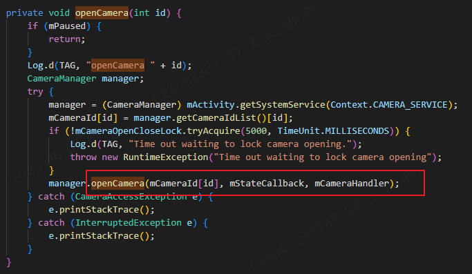
相机从app启动流程
一、流程框架图 二、具体流程分析 1、得到cameralist和对应的静态信息 目录如下: 重点代码分析: 启动相机前,先要通过getCameraIdList获取camera的个数以及id,然后可以通过getCameraCharacteristics获取对应id camera的capabilities(静态信息)进行一些openCamera前的…...

Python 包管理器 uv 介绍
Python 包管理器 uv 全面介绍 uv 是由 Astral(热门工具 Ruff 的开发者)推出的下一代高性能 Python 包管理器和构建工具,用 Rust 编写。它旨在解决传统工具(如 pip、virtualenv、pip-tools)的性能瓶颈,同时…...

高效线程安全的单例模式:Python 中的懒加载与自定义初始化参数
高效线程安全的单例模式:Python 中的懒加载与自定义初始化参数 在软件开发中,单例模式(Singleton Pattern)是一种常见的设计模式,确保一个类仅有一个实例,并提供一个全局访问点。在多线程环境下,实现单例模式时需要注意线程安全问题,以防止多个线程同时创建实例,导致…...
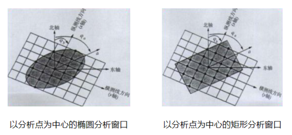
论文笔记——相干体技术在裂缝预测中的应用研究
目录 相关地震知识补充地震数据的认识地震几何属性 相干体算法定义基本原理第一代相干体技术:基于互相关的相干体技术(Correlation)第二代相干体技术:基于相似的相干体技术(Semblance)基于多道相似的相干体…...
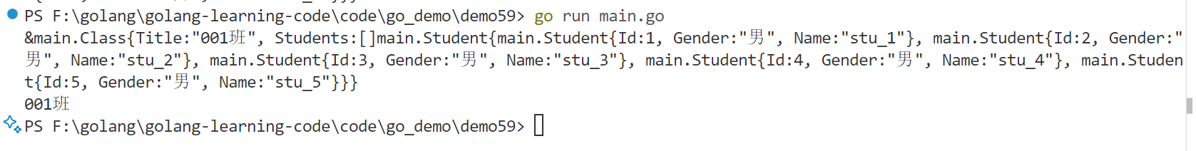
Golang——6、指针和结构体
指针和结构体 1、指针1.1、指针地址和指针类型1.2、指针取值1.3、new和make 2、结构体2.1、type关键字的使用2.2、结构体的定义和初始化2.3、结构体方法和接收者2.4、给任意类型添加方法2.5、结构体的匿名字段2.6、嵌套结构体2.7、嵌套匿名结构体2.8、结构体的继承 3、结构体与…...
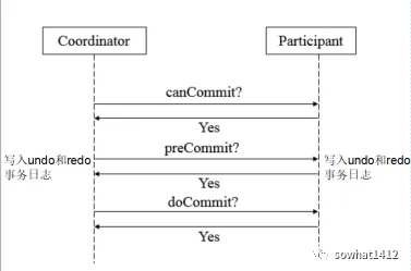
解析两阶段提交与三阶段提交的核心差异及MySQL实现方案
引言 在分布式系统的事务处理中,如何保障跨节点数据操作的一致性始终是核心挑战。经典的两阶段提交协议(2PC)通过准备阶段与提交阶段的协调机制,以同步决策模式确保事务原子性。其改进版本三阶段提交协议(3PC…...

在golang中如何将已安装的依赖降级处理,比如:将 go-ansible/v2@v2.2.0 更换为 go-ansible/@v1.1.7
在 Go 项目中降级 go-ansible 从 v2.2.0 到 v1.1.7 具体步骤: 第一步: 修改 go.mod 文件 // 原 v2 版本声明 require github.com/apenella/go-ansible/v2 v2.2.0 替换为: // 改为 v…...