使用scikit-learn为PyTorch 模型进行超参数网格搜索
scikit-learn是Python中最好的机器学习库,而PyTorch又为我们构建模型提供了方便的操作,能否将它们的优点整合起来呢?在本文中,我们将介绍如何使用 scikit-learn中的网格搜索功能来调整 PyTorch 深度学习模型的超参数:
- 如何包装 PyTorch 模型以用于 scikit-learn 以及如何使用网格搜索
- 如何网格搜索常见的神经网络参数,如学习率、Dropout、epochs、神经元数
- 在自己的项目上定义自己的超参数调优实验
如何在 scikit-learn 中使用 PyTorch 模型
要让PyTorch 模型可以在 scikit-learn 中使用的一个最简单的方法是使用skorch包。这个包为 PyTorch 模型提供与 scikit-learn 兼容的 API。 在skorch中,有分类神经网络的NeuralNetClassifier和回归神经网络的NeuralNetRegressor。
pip install skorch

要使用这些包装器,必须使用 nn.Module 将 PyTorch 模型定义为类,然后在构造 NeuralNetClassifier 类时将类的名称传递给模块参数。 例如:
class MyClassifier(nn.Module):def __init__(self):super().__init__()...def forward(self, x):...return x# create the skorch wrappermodel = NeuralNetClassifier(module=MyClassifier)
NeuralNetClassifier 类的构造函数可以获得传递给 model.fit() 调用的参数(在 scikit-learn 模型中调用训练循环的方法),例如轮次数和批量大小等。 例如:
model = NeuralNetClassifier(module=MyClassifier,max_epochs=150,batch_size=10)
NeuralNetClassifier类的构造函数也可以接受新的参数,这些参数可以传递给你的模型类的构造函数,要求是必须在它前面加上module__(两个下划线)。这些新参数可能在构造函数中带有默认值,但当包装器实例化模型时,它们将被覆盖。例如:
import torch.nn as nnfrom skorch import NeuralNetClassifierclass SonarClassifier(nn.Module):def __init__(self, n_layers=3):super().__init__()self.layers = []self.acts = []for i in range(n_layers):self.layers.append(nn.Linear(60, 60))self.acts.append(nn.ReLU())self.add_module(f"layer{i}", self.layers[-1])self.add_module(f"act{i}", self.acts[-1])self.output = nn.Linear(60, 1)def forward(self, x):for layer, act in zip(self.layers, self.acts):x = act(layer(x))x = self.output(x)return xmodel = NeuralNetClassifier(module=SonarClassifier,max_epochs=150,batch_size=10,module__n_layers=2)
我们可以通过初始化一个模型并打印来验证结果:
print(model.initialize())#结果如下:<class 'skorch.classifier.NeuralNetClassifier'>[initialized](module_=SonarClassifier((layer0): Linear(in_features=60, out_features=60, bias=True)(act0): ReLU()(layer1): Linear(in_features=60, out_features=60, bias=True)(act1): ReLU()(output): Linear(in_features=60, out_features=1, bias=True)),)
在scikit-learn中使用网格搜索
网格搜索是一种模型超参数优化技术。它只是简单地穷尽超参数的所有组合,并找到给出最佳分数的组合。在scikit-learn中,GridSearchCV类提供了这种技术。在构造这个类时,必须在param_grid参数中提供一个超参数字典。这是模型参数名和要尝试的值数组的映射。
默认使用精度作为优化的分数,但其他分数可以在GridSearchCV构造函数的score参数中指定。GridSearchCV将为每个参数组合构建一个模型进行评估。并且使用默认的3倍交叉验证,这些都是可以通过参数来进行设置的。
下面是定义一个简单网格搜索的例子:
param_grid = {'epochs': [10,20,30]}grid = GridSearchCV(estimator=model, param_grid=param_grid, n_jobs=-1, cv=3)grid_result = grid.fit(X, Y)
通过将GridSearchCV构造函数中的n_jobs参数设置为 -1表示将使用机器上的所有核心。否则,网格搜索进程将只在单线程中运行,这在多核cpu中较慢。
运行完毕就可以在grid.fit()返回的结果对象中访问网格搜索的结果。best_score提供了在优化过程中观察到的最佳分数,best_params_描述了获得最佳结果的参数组合。
示例问题描述
我们的示例都将在一个小型标准机器学习数据集上进行演示,该数据集是一个糖尿病发作分类数据集。这是一个小型数据集,所有的数值属性都很容易处理。
如何调优批大小和训练的轮次
在第一个简单示例中,我们将介绍如何调优批大小和拟合网络时使用的epoch数。
我们将简单评估从10到100的不批大小,代码清单如下所示:
import randomimport numpy as npimport torchimport torch.nn as nnimport torch.optim as optimfrom skorch import NeuralNetClassifierfrom sklearn.model_selection import GridSearchCV# load the dataset, split into input (X) and output (y) variablesdataset = np.loadtxt('pima-indians-diabetes.csv', delimiter=',')X = dataset[:,0:8]y = dataset[:,8]X = torch.tensor(X, dtype=torch.float32)y = torch.tensor(y, dtype=torch.float32).reshape(-1, 1)# PyTorch classifierclass PimaClassifier(nn.Module):def __init__(self):super().__init__()self.layer = nn.Linear(8, 12)self.act = nn.ReLU()self.output = nn.Linear(12, 1)self.prob = nn.Sigmoid()def forward(self, x):x = self.act(self.layer(x))x = self.prob(self.output(x))return x# create model with skorchmodel = NeuralNetClassifier(PimaClassifier,criterion=nn.BCELoss,optimizer=optim.Adam,verbose=False)# define the grid search parametersparam_grid = {'batch_size': [10, 20, 40, 60, 80, 100],'max_epochs': [10, 50, 100]}grid = GridSearchCV(estimator=model, param_grid=param_grid, n_jobs=-1, cv=3)grid_result = grid.fit(X, y)# summarize resultsprint("Best: %f using %s" % (grid_result.best_score_, grid_result.best_params_))means = grid_result.cv_results_['mean_test_score']stds = grid_result.cv_results_['std_test_score']params = grid_result.cv_results_['params']for mean, stdev, param in zip(means, stds, params):print("%f (%f) with: %r" % (mean, stdev, param))
结果如下:
Best: 0.714844 using {'batch_size': 10, 'max_epochs': 100}0.665365 (0.020505) with: {'batch_size': 10, 'max_epochs': 10}0.588542 (0.168055) with: {'batch_size': 10, 'max_epochs': 50}0.714844 (0.032369) with: {'batch_size': 10, 'max_epochs': 100}0.671875 (0.022326) with: {'batch_size': 20, 'max_epochs': 10}0.696615 (0.008027) with: {'batch_size': 20, 'max_epochs': 50}0.714844 (0.019918) with: {'batch_size': 20, 'max_epochs': 100}0.666667 (0.009744) with: {'batch_size': 40, 'max_epochs': 10}0.687500 (0.033603) with: {'batch_size': 40, 'max_epochs': 50}0.707031 (0.024910) with: {'batch_size': 40, 'max_epochs': 100}0.667969 (0.014616) with: {'batch_size': 60, 'max_epochs': 10}0.694010 (0.036966) with: {'batch_size': 60, 'max_epochs': 50}0.694010 (0.042473) with: {'batch_size': 60, 'max_epochs': 100}0.670573 (0.023939) with: {'batch_size': 80, 'max_epochs': 10}0.674479 (0.020752) with: {'batch_size': 80, 'max_epochs': 50}0.703125 (0.026107) with: {'batch_size': 80, 'max_epochs': 100}0.680990 (0.014382) with: {'batch_size': 100, 'max_epochs': 10}0.670573 (0.013279) with: {'batch_size': 100, 'max_epochs': 50}0.687500 (0.017758) with: {'batch_size': 100, 'max_epochs': 100}
可以看到’batch_size’: 10, ‘max_epochs’: 100达到了约71%的精度的最佳结果。
如何调整训练优化器
下面我们看看如何调整优化器,我们知道有很多个优化器可以选择比如SDG,Adam等,那么如何选择呢?
完整的代码如下:
import numpy as npimport torchimport torch.nn as nnimport torch.optim as optimfrom skorch import NeuralNetClassifierfrom sklearn.model_selection import GridSearchCV# load the dataset, split into input (X) and output (y) variablesdataset = np.loadtxt('pima-indians-diabetes.csv', delimiter=',')X = dataset[:,0:8]y = dataset[:,8]X = torch.tensor(X, dtype=torch.float32)y = torch.tensor(y, dtype=torch.float32).reshape(-1, 1)# PyTorch classifierclass PimaClassifier(nn.Module):def __init__(self):super().__init__()self.layer = nn.Linear(8, 12)self.act = nn.ReLU()self.output = nn.Linear(12, 1)self.prob = nn.Sigmoid()def forward(self, x):x = self.act(self.layer(x))x = self.prob(self.output(x))return x# create model with skorchmodel = NeuralNetClassifier(PimaClassifier,criterion=nn.BCELoss,max_epochs=100,batch_size=10,verbose=False)# define the grid search parametersparam_grid = {'optimizer': [optim.SGD, optim.RMSprop, optim.Adagrad, optim.Adadelta,optim.Adam, optim.Adamax, optim.NAdam],}grid = GridSearchCV(estimator=model, param_grid=param_grid, n_jobs=-1, cv=3)grid_result = grid.fit(X, y)# summarize resultsprint("Best: %f using %s" % (grid_result.best_score_, grid_result.best_params_))means = grid_result.cv_results_['mean_test_score']stds = grid_result.cv_results_['std_test_score']params = grid_result.cv_results_['params']for mean, stdev, param in zip(means, stds, params):print("%f (%f) with: %r" % (mean, stdev, param))
输出如下:
Best: 0.721354 using {'optimizer': <class 'torch.optim.adamax.Adamax'>}0.674479 (0.036828) with: {'optimizer': <class 'torch.optim.sgd.SGD'>}0.700521 (0.043303) with: {'optimizer': <class 'torch.optim.rmsprop.RMSprop'>}0.682292 (0.027126) with: {'optimizer': <class 'torch.optim.adagrad.Adagrad'>}0.572917 (0.051560) with: {'optimizer': <class 'torch.optim.adadelta.Adadelta'>}0.714844 (0.030758) with: {'optimizer': <class 'torch.optim.adam.Adam'>}0.721354 (0.019225) with: {'optimizer': <class 'torch.optim.adamax.Adamax'>}0.709635 (0.024360) with: {'optimizer': <class 'torch.optim.nadam.NAdam'>}
可以看到对于我们的模型和数据集Adamax优化算法是最佳的,准确率约为72%。
如何调整学习率
虽然pytorch里面学习率计划可以让我们根据轮次动态调整学习率,但是作为样例,我们将学习率和学习率的参数作为网格搜索的一个参数来进行演示。在PyTorch中,设置学习率和动量的方法如下:
optimizer = optim.SGD(lr=0.001, momentum=0.9)
在skorch包中,使用前缀optimizer__将参数路由到优化器。
import numpy as npimport torchimport torch.nn as nnimport torch.optim as optimfrom skorch import NeuralNetClassifierfrom sklearn.model_selection import GridSearchCV# load the dataset, split into input (X) and output (y) variablesdataset = np.loadtxt('pima-indians-diabetes.csv', delimiter=',')X = dataset[:,0:8]y = dataset[:,8]X = torch.tensor(X, dtype=torch.float32)y = torch.tensor(y, dtype=torch.float32).reshape(-1, 1)# PyTorch classifierclass PimaClassifier(nn.Module):def __init__(self):super().__init__()self.layer = nn.Linear(8, 12)self.act = nn.ReLU()self.output = nn.Linear(12, 1)self.prob = nn.Sigmoid()def forward(self, x):x = self.act(self.layer(x))x = self.prob(self.output(x))return x# create model with skorchmodel = NeuralNetClassifier(PimaClassifier,criterion=nn.BCELoss,optimizer=optim.SGD,max_epochs=100,batch_size=10,verbose=False)# define the grid search parametersparam_grid = {'optimizer__lr': [0.001, 0.01, 0.1, 0.2, 0.3],'optimizer__momentum': [0.0, 0.2, 0.4, 0.6, 0.8, 0.9],}grid = GridSearchCV(estimator=model, param_grid=param_grid, n_jobs=-1, cv=3)grid_result = grid.fit(X, y)# summarize resultsprint("Best: %f using %s" % (grid_result.best_score_, grid_result.best_params_))means = grid_result.cv_results_['mean_test_score']stds = grid_result.cv_results_['std_test_score']params = grid_result.cv_results_['params']for mean, stdev, param in zip(means, stds, params):print("%f (%f) with: %r" % (mean, stdev, param))
结果如下:
Best: 0.682292 using {'optimizer__lr': 0.001, 'optimizer__momentum': 0.9}0.648438 (0.016877) with: {'optimizer__lr': 0.001, 'optimizer__momentum': 0.0}0.671875 (0.017758) with: {'optimizer__lr': 0.001, 'optimizer__momentum': 0.2}0.674479 (0.022402) with: {'optimizer__lr': 0.001, 'optimizer__momentum': 0.4}0.677083 (0.011201) with: {'optimizer__lr': 0.001, 'optimizer__momentum': 0.6}0.679688 (0.027621) with: {'optimizer__lr': 0.001, 'optimizer__momentum': 0.8}0.682292 (0.026557) with: {'optimizer__lr': 0.001, 'optimizer__momentum': 0.9}0.671875 (0.019918) with: {'optimizer__lr': 0.01, 'optimizer__momentum': 0.0}0.648438 (0.024910) with: {'optimizer__lr': 0.01, 'optimizer__momentum': 0.2}0.546875 (0.143454) with: {'optimizer__lr': 0.01, 'optimizer__momentum': 0.4}0.567708 (0.153668) with: {'optimizer__lr': 0.01, 'optimizer__momentum': 0.6}0.552083 (0.141790) with: {'optimizer__lr': 0.01, 'optimizer__momentum': 0.8}0.451823 (0.144561) with: {'optimizer__lr': 0.01, 'optimizer__momentum': 0.9}0.348958 (0.001841) with: {'optimizer__lr': 0.1, 'optimizer__momentum': 0.0}0.450521 (0.142719) with: {'optimizer__lr': 0.1, 'optimizer__momentum': 0.2}0.450521 (0.142719) with: {'optimizer__lr': 0.1, 'optimizer__momentum': 0.4}0.450521 (0.142719) with: {'optimizer__lr': 0.1, 'optimizer__momentum': 0.6}0.348958 (0.001841) with: {'optimizer__lr': 0.1, 'optimizer__momentum': 0.8}0.348958 (0.001841) with: {'optimizer__lr': 0.1, 'optimizer__momentum': 0.9}0.444010 (0.136265) with: {'optimizer__lr': 0.2, 'optimizer__momentum': 0.0}0.450521 (0.142719) with: {'optimizer__lr': 0.2, 'optimizer__momentum': 0.2}0.348958 (0.001841) with: {'optimizer__lr': 0.2, 'optimizer__momentum': 0.4}0.552083 (0.141790) with: {'optimizer__lr': 0.2, 'optimizer__momentum': 0.6}0.549479 (0.142719) with: {'optimizer__lr': 0.2, 'optimizer__momentum': 0.8}0.651042 (0.001841) with: {'optimizer__lr': 0.2, 'optimizer__momentum': 0.9}0.552083 (0.141790) with: {'optimizer__lr': 0.3, 'optimizer__momentum': 0.0}0.348958 (0.001841) with: {'optimizer__lr': 0.3, 'optimizer__momentum': 0.2}0.450521 (0.142719) with: {'optimizer__lr': 0.3, 'optimizer__momentum': 0.4}0.552083 (0.141790) with: {'optimizer__lr': 0.3, 'optimizer__momentum': 0.6}0.450521 (0.142719) with: {'optimizer__lr': 0.3, 'optimizer__momentum': 0.8}0.450521 (0.142719) with: {'optimizer__lr': 0.3, 'optimizer__momentum': 0.9}
对于SGD,使用0.001的学习率和0.9的动量获得了最佳结果,准确率约为68%。
如何激活函数
激活函数控制单个神经元的非线性。我们将演示评估PyTorch中可用的一些激活函数。
import numpy as npimport torchimport torch.nn as nnimport torch.nn.init as initimport torch.optim as optimfrom skorch import NeuralNetClassifierfrom sklearn.model_selection import GridSearchCV# load the dataset, split into input (X) and output (y) variablesdataset = np.loadtxt('pima-indians-diabetes.csv', delimiter=',')X = dataset[:,0:8]y = dataset[:,8]X = torch.tensor(X, dtype=torch.float32)y = torch.tensor(y, dtype=torch.float32).reshape(-1, 1)# PyTorch classifierclass PimaClassifier(nn.Module):def __init__(self, activation=nn.ReLU):super().__init__()self.layer = nn.Linear(8, 12)self.act = activation()self.output = nn.Linear(12, 1)self.prob = nn.Sigmoid()# manually init weightsinit.kaiming_uniform_(self.layer.weight)init.kaiming_uniform_(self.output.weight)def forward(self, x):x = self.act(self.layer(x))x = self.prob(self.output(x))return x# create model with skorchmodel = NeuralNetClassifier(PimaClassifier,criterion=nn.BCELoss,optimizer=optim.Adamax,max_epochs=100,batch_size=10,verbose=False)# define the grid search parametersparam_grid = {'module__activation': [nn.Identity, nn.ReLU, nn.ELU, nn.ReLU6,nn.GELU, nn.Softplus, nn.Softsign, nn.Tanh,nn.Sigmoid, nn.Hardsigmoid]}grid = GridSearchCV(estimator=model, param_grid=param_grid, n_jobs=-1, cv=3)grid_result = grid.fit(X, y)# summarize resultsprint("Best: %f using %s" % (grid_result.best_score_, grid_result.best_params_))means = grid_result.cv_results_['mean_test_score']stds = grid_result.cv_results_['std_test_score']params = grid_result.cv_results_['params']for mean, stdev, param in zip(means, stds, params):print("%f (%f) with: %r" % (mean, stdev, param))
结果如下:
Best: 0.699219 using {'module__activation': <class 'torch.nn.modules.activation.ReLU'>}0.687500 (0.025315) with: {'module__activation': <class 'torch.nn.modules.linear.Identity'>}0.699219 (0.011049) with: {'module__activation': <class 'torch.nn.modules.activation.ReLU'>}0.674479 (0.035849) with: {'module__activation': <class 'torch.nn.modules.activation.ELU'>}0.621094 (0.063549) with: {'module__activation': <class 'torch.nn.modules.activation.ReLU6'>}0.674479 (0.017566) with: {'module__activation': <class 'torch.nn.modules.activation.GELU'>}0.558594 (0.149189) with: {'module__activation': <class 'torch.nn.modules.activation.Softplus'>}0.675781 (0.014616) with: {'module__activation': <class 'torch.nn.modules.activation.Softsign'>}0.619792 (0.018688) with: {'module__activation': <class 'torch.nn.modules.activation.Tanh'>}0.643229 (0.019225) with: {'module__activation': <class 'torch.nn.modules.activation.Sigmoid'>}0.636719 (0.022326) with: {'module__activation': <class 'torch.nn.modules.activation.Hardsigmoid'>}
ReLU激活函数获得了最好的结果,准确率约为70%。
如何调整Dropout参数
在本例中,我们将尝试在0.0到0.9之间的dropout百分比(1.0没有意义)和在0到5之间的MaxNorm权重约束值。
import numpy as npimport torchimport torch.nn as nnimport torch.nn.init as initimport torch.optim as optimfrom skorch import NeuralNetClassifierfrom sklearn.model_selection import GridSearchCV# load the dataset, split into input (X) and output (y) variablesdataset = np.loadtxt('pima-indians-diabetes.csv', delimiter=',')X = dataset[:,0:8]y = dataset[:,8]X = torch.tensor(X, dtype=torch.float32)y = torch.tensor(y, dtype=torch.float32).reshape(-1, 1)# PyTorch classifierclass PimaClassifier(nn.Module):def __init__(self, dropout_rate=0.5, weight_constraint=1.0):super().__init__()self.layer = nn.Linear(8, 12)self.act = nn.ReLU()self.dropout = nn.Dropout(dropout_rate)self.output = nn.Linear(12, 1)self.prob = nn.Sigmoid()self.weight_constraint = weight_constraint# manually init weightsinit.kaiming_uniform_(self.layer.weight)init.kaiming_uniform_(self.output.weight)def forward(self, x):# maxnorm weight before actual forward passwith torch.no_grad():norm = self.layer.weight.norm(2, dim=0, keepdim=True).clamp(min=self.weight_constraint / 2)desired = torch.clamp(norm, max=self.weight_constraint)self.layer.weight *= (desired / norm)# actual forward passx = self.act(self.layer(x))x = self.dropout(x)x = self.prob(self.output(x))return x# create model with skorchmodel = NeuralNetClassifier(PimaClassifier,criterion=nn.BCELoss,optimizer=optim.Adamax,max_epochs=100,batch_size=10,verbose=False)# define the grid search parametersparam_grid = {'module__weight_constraint': [1.0, 2.0, 3.0, 4.0, 5.0],'module__dropout_rate': [0.0, 0.1, 0.2, 0.3, 0.4, 0.5, 0.6, 0.7, 0.8, 0.9]}grid = GridSearchCV(estimator=model, param_grid=param_grid, n_jobs=-1, cv=3)grid_result = grid.fit(X, y)# summarize resultsprint("Best: %f using %s" % (grid_result.best_score_, grid_result.best_params_))means = grid_result.cv_results_['mean_test_score']stds = grid_result.cv_results_['std_test_score']params = grid_result.cv_results_['params']for mean, stdev, param in zip(means, stds, params):print("%f (%f) with: %r" % (mean, stdev, param))
结果如下:
Best: 0.701823 using {'module__dropout_rate': 0.1, 'module__weight_constraint': 2.0}0.669271 (0.015073) with: {'module__dropout_rate': 0.0, 'module__weight_constraint': 1.0}0.692708 (0.035132) with: {'module__dropout_rate': 0.0, 'module__weight_constraint': 2.0}0.589844 (0.170180) with: {'module__dropout_rate': 0.0, 'module__weight_constraint': 3.0}0.561198 (0.151131) with: {'module__dropout_rate': 0.0, 'module__weight_constraint': 4.0}0.688802 (0.021710) with: {'module__dropout_rate': 0.0, 'module__weight_constraint': 5.0}0.697917 (0.009744) with: {'module__dropout_rate': 0.1, 'module__weight_constraint': 1.0}0.701823 (0.016367) with: {'module__dropout_rate': 0.1, 'module__weight_constraint': 2.0}0.694010 (0.010253) with: {'module__dropout_rate': 0.1, 'module__weight_constraint': 3.0}0.686198 (0.025976) with: {'module__dropout_rate': 0.1, 'module__weight_constraint': 4.0}0.679688 (0.026107) with: {'module__dropout_rate': 0.1, 'module__weight_constraint': 5.0}0.701823 (0.029635) with: {'module__dropout_rate': 0.2, 'module__weight_constraint': 1.0}0.682292 (0.014731) with: {'module__dropout_rate': 0.2, 'module__weight_constraint': 2.0}0.701823 (0.009744) with: {'module__dropout_rate': 0.2, 'module__weight_constraint': 3.0}0.701823 (0.026557) with: {'module__dropout_rate': 0.2, 'module__weight_constraint': 4.0}0.687500 (0.015947) with: {'module__dropout_rate': 0.2, 'module__weight_constraint': 5.0}0.686198 (0.006639) with: {'module__dropout_rate': 0.3, 'module__weight_constraint': 1.0}0.656250 (0.006379) with: {'module__dropout_rate': 0.3, 'module__weight_constraint': 2.0}0.565104 (0.155608) with: {'module__dropout_rate': 0.3, 'module__weight_constraint': 3.0}0.700521 (0.028940) with: {'module__dropout_rate': 0.3, 'module__weight_constraint': 4.0}0.669271 (0.012890) with: {'module__dropout_rate': 0.3, 'module__weight_constraint': 5.0}0.661458 (0.018688) with: {'module__dropout_rate': 0.4, 'module__weight_constraint': 1.0}0.669271 (0.017566) with: {'module__dropout_rate': 0.4, 'module__weight_constraint': 2.0}0.652344 (0.006379) with: {'module__dropout_rate': 0.4, 'module__weight_constraint': 3.0}0.680990 (0.037783) with: {'module__dropout_rate': 0.4, 'module__weight_constraint': 4.0}0.692708 (0.042112) with: {'module__dropout_rate': 0.4, 'module__weight_constraint': 5.0}0.666667 (0.006639) with: {'module__dropout_rate': 0.5, 'module__weight_constraint': 1.0}0.652344 (0.011500) with: {'module__dropout_rate': 0.5, 'module__weight_constraint': 2.0}0.662760 (0.007366) with: {'module__dropout_rate': 0.5, 'module__weight_constraint': 3.0}0.558594 (0.146610) with: {'module__dropout_rate': 0.5, 'module__weight_constraint': 4.0}0.552083 (0.141826) with: {'module__dropout_rate': 0.5, 'module__weight_constraint': 5.0}0.548177 (0.141826) with: {'module__dropout_rate': 0.6, 'module__weight_constraint': 1.0}0.653646 (0.013279) with: {'module__dropout_rate': 0.6, 'module__weight_constraint': 2.0}0.661458 (0.008027) with: {'module__dropout_rate': 0.6, 'module__weight_constraint': 3.0}0.553385 (0.142719) with: {'module__dropout_rate': 0.6, 'module__weight_constraint': 4.0}0.669271 (0.035132) with: {'module__dropout_rate': 0.6, 'module__weight_constraint': 5.0}0.662760 (0.015733) with: {'module__dropout_rate': 0.7, 'module__weight_constraint': 1.0}0.636719 (0.024910) with: {'module__dropout_rate': 0.7, 'module__weight_constraint': 2.0}0.550781 (0.146818) with: {'module__dropout_rate': 0.7, 'module__weight_constraint': 3.0}0.537760 (0.140094) with: {'module__dropout_rate': 0.7, 'module__weight_constraint': 4.0}0.542969 (0.138144) with: {'module__dropout_rate': 0.7, 'module__weight_constraint': 5.0}0.565104 (0.148654) with: {'module__dropout_rate': 0.8, 'module__weight_constraint': 1.0}0.657552 (0.008027) with: {'module__dropout_rate': 0.8, 'module__weight_constraint': 2.0}0.428385 (0.111418) with: {'module__dropout_rate': 0.8, 'module__weight_constraint': 3.0}0.549479 (0.142719) with: {'module__dropout_rate': 0.8, 'module__weight_constraint': 4.0}0.648438 (0.005524) with: {'module__dropout_rate': 0.8, 'module__weight_constraint': 5.0}0.540365 (0.136861) with: {'module__dropout_rate': 0.9, 'module__weight_constraint': 1.0}0.605469 (0.053083) with: {'module__dropout_rate': 0.9, 'module__weight_constraint': 2.0}0.553385 (0.139948) with: {'module__dropout_rate': 0.9, 'module__weight_constraint': 3.0}0.549479 (0.142719) with: {'module__dropout_rate': 0.9, 'module__weight_constraint': 4.0}0.595052 (0.075566) with: {'module__dropout_rate': 0.9, 'module__weight_constraint': 5.0}
可以看到,10%的Dropout和2.0的权重约束获得了70%的最佳精度。
如何调整隐藏层神经元的数量
单层神经元的数量是一个需要调优的重要参数。一般来说,一层神经元的数量控制着网络的表示能力,至少在拓扑的这一点上是这样。
理论上来说:由于通用逼近定理,一个足够大的单层网络可以近似任何其他神经网络。
在本例中,将尝试从1到30的值,步骤为5。一个更大的网络需要更多的训练,至少批大小和epoch的数量应该与神经元的数量一起优化。
import numpy as npimport torchimport torch.nn as nnimport torch.nn.init as initimport torch.optim as optimfrom skorch import NeuralNetClassifierfrom sklearn.model_selection import GridSearchCV# load the dataset, split into input (X) and output (y) variablesdataset = np.loadtxt('pima-indians-diabetes.csv', delimiter=',')X = dataset[:,0:8]y = dataset[:,8]X = torch.tensor(X, dtype=torch.float32)y = torch.tensor(y, dtype=torch.float32).reshape(-1, 1)class PimaClassifier(nn.Module):def __init__(self, n_neurons=12):super().__init__()self.layer = nn.Linear(8, n_neurons)self.act = nn.ReLU()self.dropout = nn.Dropout(0.1)self.output = nn.Linear(n_neurons, 1)self.prob = nn.Sigmoid()self.weight_constraint = 2.0# manually init weightsinit.kaiming_uniform_(self.layer.weight)init.kaiming_uniform_(self.output.weight)def forward(self, x):# maxnorm weight before actual forward passwith torch.no_grad():norm = self.layer.weight.norm(2, dim=0, keepdim=True).clamp(min=self.weight_constraint / 2)desired = torch.clamp(norm, max=self.weight_constraint)self.layer.weight *= (desired / norm)# actual forward passx = self.act(self.layer(x))x = self.dropout(x)x = self.prob(self.output(x))return x# create model with skorchmodel = NeuralNetClassifier(PimaClassifier,criterion=nn.BCELoss,optimizer=optim.Adamax,max_epochs=100,batch_size=10,verbose=False)# define the grid search parametersparam_grid = {'module__n_neurons': [1, 5, 10, 15, 20, 25, 30]}grid = GridSearchCV(estimator=model, param_grid=param_grid, n_jobs=-1, cv=3)grid_result = grid.fit(X, y)# summarize resultsprint("Best: %f using %s" % (grid_result.best_score_, grid_result.best_params_))means = grid_result.cv_results_['mean_test_score']stds = grid_result.cv_results_['std_test_score']params = grid_result.cv_results_['params']for mean, stdev, param in zip(means, stds, params):print("%f (%f) with: %r" % (mean, stdev, param))
结果如下:
Best: 0.708333 using {'module__n_neurons': 30}0.654948 (0.003683) with: {'module__n_neurons': 1}0.666667 (0.023073) with: {'module__n_neurons': 5}0.694010 (0.014382) with: {'module__n_neurons': 10}0.682292 (0.014382) with: {'module__n_neurons': 15}0.707031 (0.028705) with: {'module__n_neurons': 20}0.703125 (0.030758) with: {'module__n_neurons': 25}0.708333 (0.015733) with: {'module__n_neurons': 30}
你可以看到,在隐藏层中有30个神经元的网络获得了最好的结果,准确率约为71%。
总结
在这篇文章中,我们介绍了如何使用PyTorch和scikit-learn在Python中优化深度学习网络的超参数。如果你对skorch 感兴趣,可以看看他的文档
https://avoid.overfit.cn/post/fda8764b85174b6ca3c9eac4fc6d0db9
作者:Jason Brownlee
相关文章:
使用scikit-learn为PyTorch 模型进行超参数网格搜索
scikit-learn是Python中最好的机器学习库,而PyTorch又为我们构建模型提供了方便的操作,能否将它们的优点整合起来呢?在本文中,我们将介绍如何使用 scikit-learn中的网格搜索功能来调整 PyTorch 深度学习模型的超参数: 如何包装 P…...

Windeployqt 打包,缺少dll 的解决方法
Windeployqt 打包,缺少DLL 的原因分析,解决方法 很多同学使用工具windeployqt进行打包发布后,运行exe文件时,还是会出现下图所示的系统错误提示,这种情况就表示相关的DLL 库文件没有被正确打包。可是windeployqt明确显…...

第四章:搭建Windows server AD域和树域
由于Windows简单一点,我就先搞Windows了。AD域:视频教程:https://www.bilibili.com/video/BV1f84y1G72x/在创建AD域时要把网卡配置好这是打开网卡界面的命令DNS要改成自己的,因为在创建域的同时也会自动创建DNS打开服务器管理器&a…...

【解决方案】老旧小区升级改造,视频智能化能力如何提升居民安全感?
一、需求背景 随着我国社会经济的快速发展与进步,城市宜居程度成为城市发展的重要指标,城市的发展面临着更新、改造和宜居建设等。一方面,社区居民对生活的环境提出了更高的要求;另一方面,将“智慧城市”的概念引入社…...

【遇见青山】项目难点:缓存穿透的解决方案
【遇见青山】项目难点:缓存穿透的解决方案1.缓存穿透现象缓存空对象布隆过滤其他方案2.解决方案,缓存空数据1.缓存穿透现象 缓存穿透是指客户端请求的数据在缓存中和数据库中都不存在,这样缓存永远不会生效,这些请求都会打到数据…...

单一职责原则|SOLID as a rock
文章目录 意图动机:违反单一职责原则解决方案:C++中单一职责原则的例子单一职责的优点1、可理解性2、可维护性3、可复用性在C++中用好SRP的标准总结本文是关于 SOLID as Rock 设计原则系列的五部分中的第一部分。 SOLID 设计原则侧重于开发 易于维护、可重用和可扩展的软件。…...

使用百度地图官方WEB API,提示 “ APP 服务被禁用“ 问题的解决方法
问题描述 项目上用了百度地图官方WEB API,打开界面时百度地图无法打开,出现弹窗: APP被您禁用啦。详情查看:http://lbsyun.baidu.com/apiconsole/key#。 原因分析: 查看错误信息:"status":240,…...

nodejs如何实现Digest摘要认证?
文章目录1.前言2. 原理3. 过程4. node实现摘要认证5. 前端如何Digest摘要登录认证(下面是海康的设备代码)1.前言 根据项目需求,海康设备ISAPI协议需要摘要认证,那么什么是摘要认证?估计不少搞到几年的前端连摘要认证都…...

【C#项目】图书馆管理系统-WinForm+MySQL
文章目录前言一、业务梳理与需求分析1.功能描述2.实现步骤3.功能逻辑图二、数据库设计1.实体-关系(E-R图)概念模型设计2.数据表设计三、WinForm界面交互设计1、界面交互逻辑2、项目树3、主界面登录界面4、 图书查询界面5、图书借阅界面6、图书插入界面7、…...
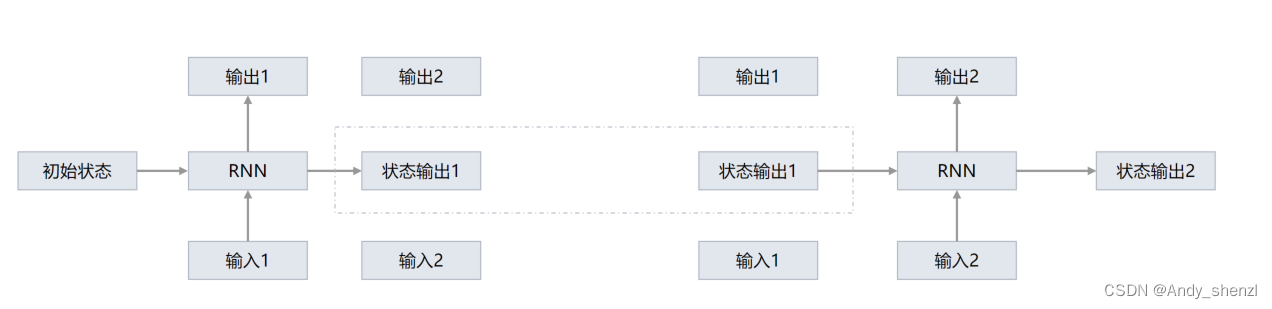
RNN循环神经网络原理理解
一、基础 正常的神经网络 一般情况下,输入层提供数据,全连接进入隐藏层,隐藏层可以是多层,层与层之间是全连接,最后输出到输出层;通过不断的调整权重参数和偏置参数实现训练的效果。深度学习的网络都是水…...

一句话设计模式1: 单例模式
单例模式:全局唯一的对象。 文章目录 单例模式:全局唯一的对象。前言一、为什么要全局唯一?二、如何实现单例1. 注入到spring中2. 饿汉式3. 懒汉式第一种: 静态内部类第二种: synchronized 关键字第二种: 双重锁检查总结前言 单例可以说是设计模式中很常用的模式了,但也可以说…...

新版国家标准GB/T 28181—2022将于2023年7月1日正式实施,与GB/T 28181—2016差别有哪些?
新版国家标准GB/T28181-2022《公共安全视频监控联网系统信息传输、交换、控制技术要求》已于2022年12月30日发布,将于2023年7月1日正式实施。与GB/T 28181—2016相比,除结构调整和编辑性改动外,主要技术变化如下。——更改了标准范围…...
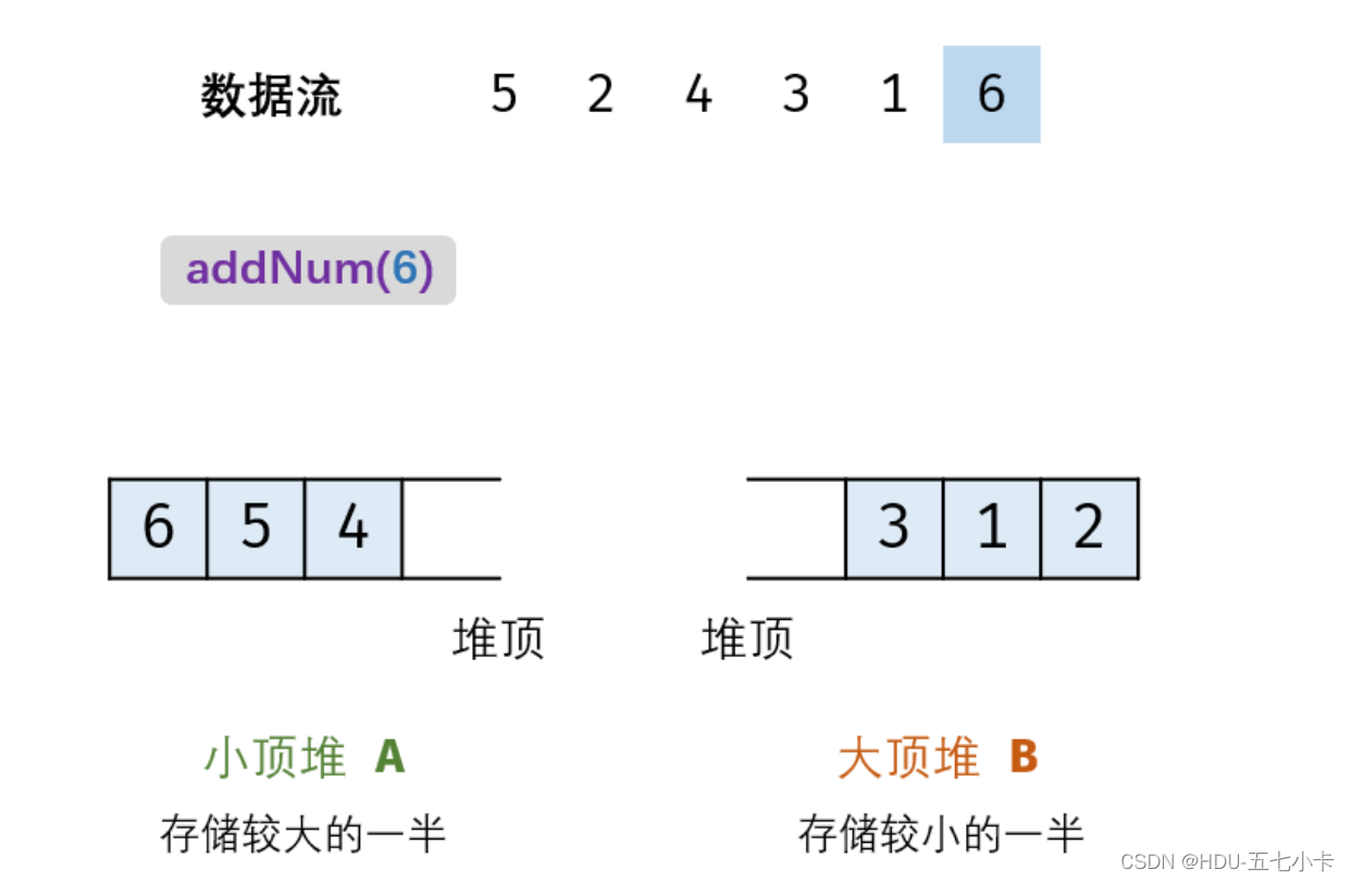
剑指 Offer 41. 数据流中的中位数
题目 如何得到一个数据流中的中位数?如果从数据流中读出奇数个数值,那么中位数就是所有数值排序之后位于中间的数值。如果从数据流中读出偶数个数值,那么中位数就是所有数值排序之后中间两个数的平均值。 例如,[2,3,4] 的中位数是…...

分布式架构下,Session共享有什么方案?
分布式架构下,Session共享有什么方案? 1.不要有Session:但是确实在某些场景下,是可以没有session的,其实在很多借口类系统当中,都提倡【API无状态服务】; 也就是每一次的接口访问,都…...

瀚博半导体载天VA1 加速卡安装过程
背景: 想用 瀚博半导体载天VA1 加速卡 代替 NVIDIA 显卡跑深度学习模型 感谢瀚博的周工帮助解答。 正文: 小心拔出 NVIDIA 显卡,在PCIe 接口插上瀚博半导体载天VA1加速卡,如图: 这时显示屏连接主板的集成显卡 卸载…...

服务降级和熔断机制
🏆今日学习目标: 🍀服务降级和熔断机制 ✅创作者:林在闪闪发光 ⏰预计时间:30分钟 🎉个人主页:林在闪闪发光的个人主页 🍁林在闪闪发光的个人社区,欢迎你的加入: 林在闪闪…...

史上最全最详细的Instagram 欢迎消息引流及示例
史上最全最详细的Instagram 欢迎消息引流及示例!关键词: Instagram 欢迎消息SaleSmartly(ss客服) 寻找 Instagram 欢迎消息示例,您可以用于您的业务。在本文中,我们将介绍Instagram欢迎消息的基础知识和好处…...

MDB 5 UI-KIT Bootstrap 5 最新版放送
顶级开源 UI 套件,Bootstrap v5 和 v4 的材料设计,jQuery 版本,数百个优质组件和模板,所有一致的,有据可查的,可靠的超级简单,1分钟安装简单的主题和定制 受到超过 3,000,000 名开发人员和设计师…...

做专家型服务者,尚博信助力企业数字化转型跑出“加速度” | 爱分析调研
01 从技术应用到业务重构,数字化市场呼唤专家型厂商 企业数字化转型是一个长期且系统性的变革过程。伴随着企业从信息化建设转向业务的数字化重构,市场对数字化厂商的能力要求也在升级。 早期的信息化建设主要是从技术视角切入,采用局部需求…...

CSS 重新认识 !important 肯定有你不知道的
重新认识 !important 影响级联规则 与 animation 和 transition 的关系级联层cascade layer内联样式!important 与权重 !important 与简写属性!important 与自定义变量!important 最佳实践 在开始之前, 先来规范一下文中的用于, 首先看 W3C 中关于 CSS 的一些术语定义吧. 下图…...

docker详细操作--未完待续
docker介绍 docker官网: Docker:加速容器应用程序开发 harbor官网:Harbor - Harbor 中文 使用docker加速器: Docker镜像极速下载服务 - 毫秒镜像 是什么 Docker 是一种开源的容器化平台,用于将应用程序及其依赖项(如库、运行时环…...
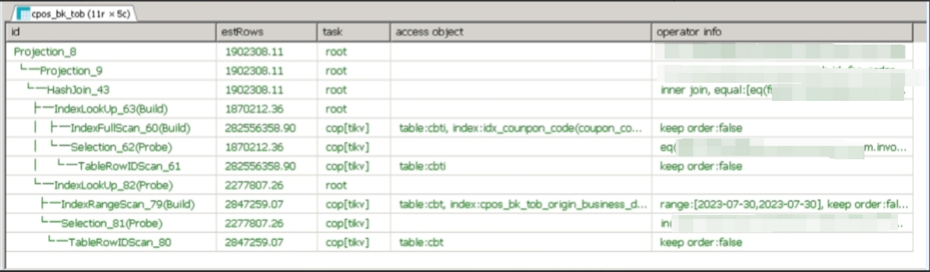
【入坑系列】TiDB 强制索引在不同库下不生效问题
文章目录 背景SQL 优化情况线上SQL运行情况分析怀疑1:执行计划绑定问题?尝试:SHOW WARNINGS 查看警告探索 TiDB 的 USE_INDEX 写法Hint 不生效问题排查解决参考背景 项目中使用 TiDB 数据库,并对 SQL 进行优化了,添加了强制索引。 UAT 环境已经生效,但 PROD 环境强制索…...

智能在线客服平台:数字化时代企业连接用户的 AI 中枢
随着互联网技术的飞速发展,消费者期望能够随时随地与企业进行交流。在线客服平台作为连接企业与客户的重要桥梁,不仅优化了客户体验,还提升了企业的服务效率和市场竞争力。本文将探讨在线客服平台的重要性、技术进展、实际应用,并…...
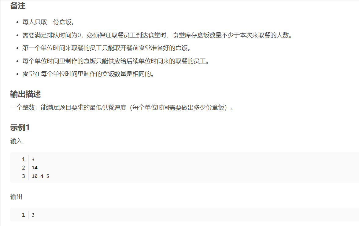
华为OD机试-食堂供餐-二分法
import java.util.Arrays; import java.util.Scanner;public class DemoTest3 {public static void main(String[] args) {Scanner in new Scanner(System.in);// 注意 hasNext 和 hasNextLine 的区别while (in.hasNextLine()) { // 注意 while 处理多个 caseint a in.nextIn…...
SpringBoot+uniapp 的 Champion 俱乐部微信小程序设计与实现,论文初版实现
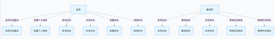
摘要 本论文旨在设计并实现基于 SpringBoot 和 uniapp 的 Champion 俱乐部微信小程序,以满足俱乐部线上活动推广、会员管理、社交互动等需求。通过 SpringBoot 搭建后端服务,提供稳定高效的数据处理与业务逻辑支持;利用 uniapp 实现跨平台前…...

高危文件识别的常用算法:原理、应用与企业场景
高危文件识别的常用算法:原理、应用与企业场景 高危文件识别旨在检测可能导致安全威胁的文件,如包含恶意代码、敏感数据或欺诈内容的文档,在企业协同办公环境中(如Teams、Google Workspace)尤为重要。结合大模型技术&…...
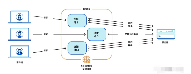
Cloudflare 从 Nginx 到 Pingora:性能、效率与安全的全面升级
在互联网的快速发展中,高性能、高效率和高安全性的网络服务成为了各大互联网基础设施提供商的核心追求。Cloudflare 作为全球领先的互联网安全和基础设施公司,近期做出了一个重大技术决策:弃用长期使用的 Nginx,转而采用其内部开发…...
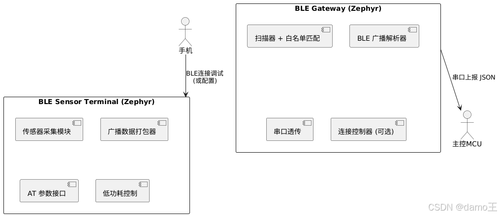
【Zephyr 系列 10】实战项目:打造一个蓝牙传感器终端 + 网关系统(完整架构与全栈实现)
🧠关键词:Zephyr、BLE、终端、网关、广播、连接、传感器、数据采集、低功耗、系统集成 📌目标读者:希望基于 Zephyr 构建 BLE 系统架构、实现终端与网关协作、具备产品交付能力的开发者 📊篇幅字数:约 5200 字 ✨ 项目总览 在物联网实际项目中,**“终端 + 网关”**是…...
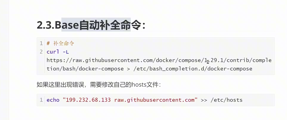
(转)什么是DockerCompose?它有什么作用?
一、什么是DockerCompose? DockerCompose可以基于Compose文件帮我们快速的部署分布式应用,而无需手动一个个创建和运行容器。 Compose文件是一个文本文件,通过指令定义集群中的每个容器如何运行。 DockerCompose就是把DockerFile转换成指令去运行。 …...

实现弹窗随键盘上移居中
实现弹窗随键盘上移的核心思路 在Android中,可以通过监听键盘的显示和隐藏事件,动态调整弹窗的位置。关键点在于获取键盘高度,并计算剩余屏幕空间以重新定位弹窗。 // 在Activity或Fragment中设置键盘监听 val rootView findViewById<V…...