R_handbook_作图专题
ggplot基本作图
1 条形图
library(ggplot2)
ggplot(biopics) + geom_histogram(aes(x = year_release),binwidth=1,fill="gray")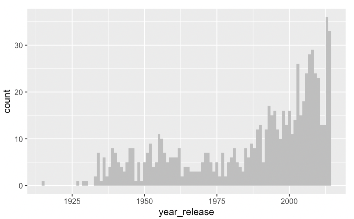
2 堆砌柱状图
ggplot(biopics, aes(x=year_release)) +geom_bar(aes(fill=subject_sex))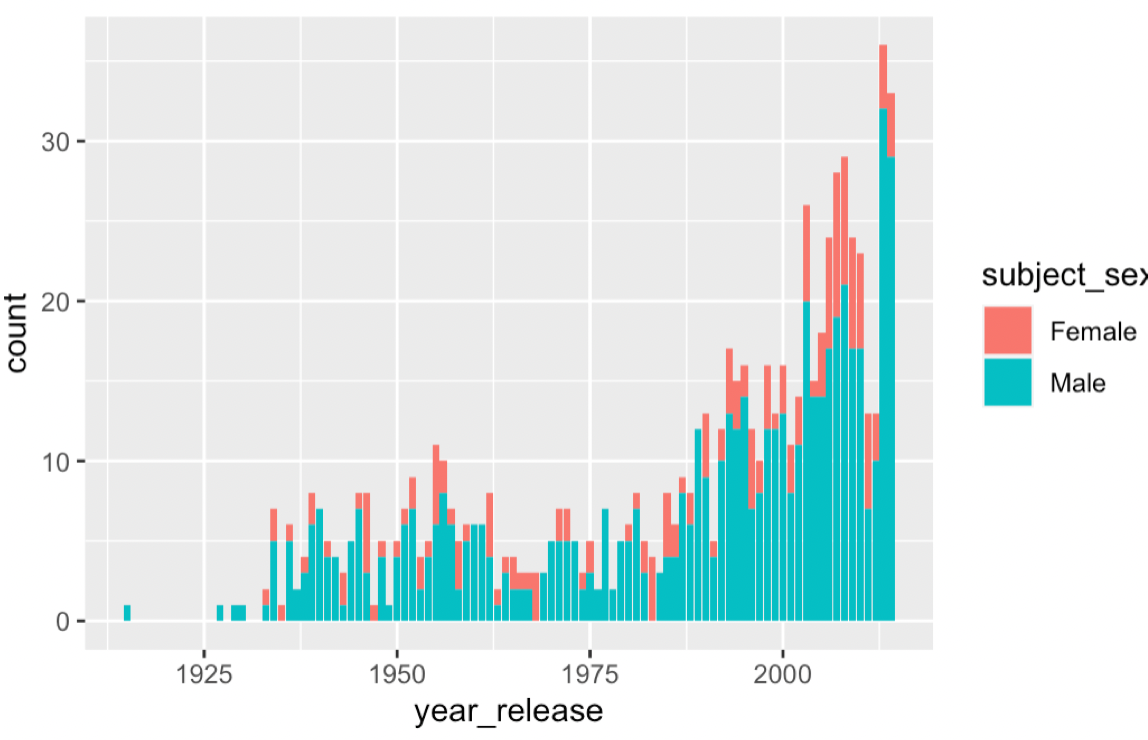
3 堆砌比例柱状图
ggplot(biopics, aes(x=year_release)) +geom_bar(aes(fill=subject_sex),position = 'fill')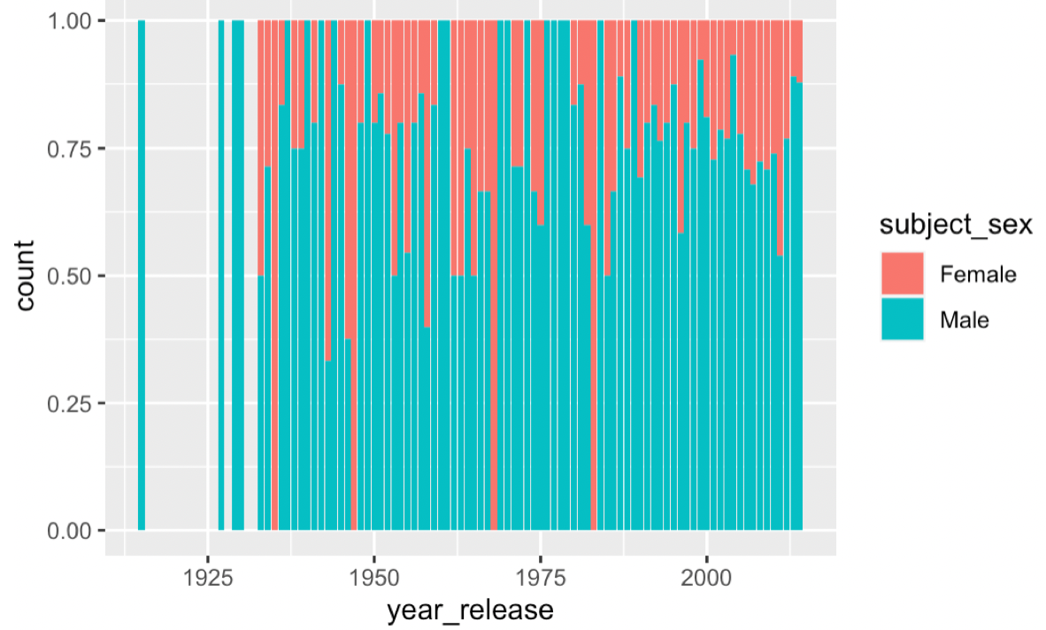
4 马赛克图
library(vcd)
bio_ques_d <- biopics[,c(11,13)]
bio_ques_d$subject_race <- ifelse(is.na(bio_ques_d$subject_race ), "missing",ifelse(bio_ques_d$subject_race == "White","White", "nonwhite"))
biq_ques_d_table <- table(bio_ques_d$subject_race,bio_ques_d$subject_sex)
mosaicplot(biq_ques_d_table)
5 双散点图
process_var <- c('v32', 'v33', 'v34', 'v35', 'v36', 'v37')
for (i in c(1:6)){var_clean <- paste(process_var[i],'clean',sep = '_')data[,var_clean] <- ifelse(data[,process_var[i]] == 'trust completely',1,ifelse(data[,process_var[i]] == 'trust somewhat',2,ifelse(data[,process_var[i]] == 'do not trust very much',3,ifelse(data[,process_var[i]] == 'do not trust at all',4,NA))))
}
data$intp.trust <- rowSums(data[,c(438:443)],na.rm = TRUE)
data$intp.trust <- data$intp.trust/6
ggplot(data[data$country == 'Iceland',], aes(x=confidence, y=intp.trust, colour=v225)) + geom_point()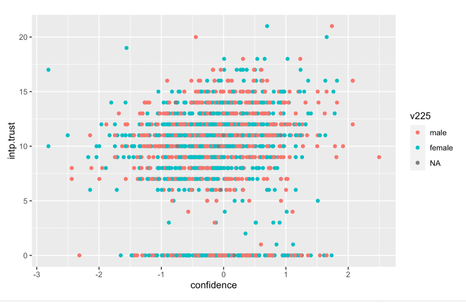
6 双密度图
ggplot(data=start_s_country_data) +geom_density(aes(x=residual,color=as.factor(v225),))## 自定义图例的情况
ggplot(data=data) +geom_density(aes(x=LW, color = "LW")) + geom_density(aes(x=LP, color = "LP")) + labs(title="") + xlab("Value") + theme(legend.title=element_blank(),legend.position = c(0.9, 0.9))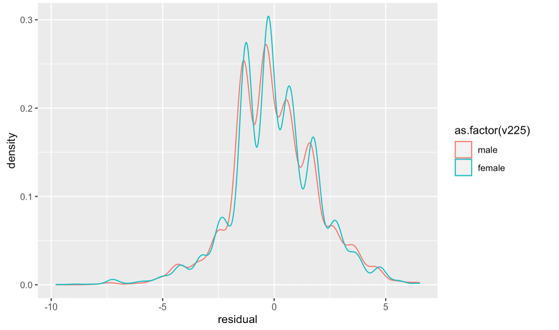
ggplot(data ) +geom_point(aes(x = No.education, y=Median.year.of.schooling)) + geom_smooth(aes(x = No.education, y=Median.year.of.schooling), method = 'lm') + theme_classic() 7 双折线图与多图展示
library(dplyr)
library(devtools)
library(cowplot)plot_grid(plot1,plot3,plot5,plot2,plot4,plot6,ncol=3,nrow=2)
bio_ques_f <- biopics[,c(4,11,13)]
bio_ques_f$subject_race <- ifelse(is.na(bio_ques_f$subject_race ), "missing",ifelse(bio_ques_f$subject_race == "White","White", "nonwhite"))planes <- group_by(bio_ques_f, year_release, subject_race, subject_sex)
bio_ques_f_summary <- summarise(planes, count = n())
planes <- group_by(bio_ques_f,year_release)
bio_ques_f_year<- summarise(planes,count_year = n())bio_ques_f_summary <- left_join(bio_ques_f_summary,bio_ques_f_year,c("year_release" = "year_release"))
bio_ques_f_summary$prop <- bio_ques_f_summary$count / bio_ques_f_summary$count_yeardata_missing_female <- subset(bio_ques_f_summary,with(bio_ques_f_summary,(subject_race == 'missing') & (subject_sex == 'Female')))
data_missing_male <- subset(bio_ques_f_summary,with(bio_ques_f_summary,(subject_race == 'missing') & (subject_sex == 'Male')))
data_nonwhite_female <- subset(bio_ques_f_summary,with(bio_ques_f_summary,(subject_race == 'nonwhite') & (subject_sex == 'Female')))
data_nonwhite_male <- subset(bio_ques_f_summary,with(bio_ques_f_summary,(subject_race == 'nonwhite') & (subject_sex == 'Male')))
data_white_female <- subset(bio_ques_f_summary,with(bio_ques_f_summary,(subject_race == 'White') & (subject_sex == 'Female')))
data_white_male <- subset(bio_ques_f_summary,with(bio_ques_f_summary,(subject_race == 'White') & (subject_sex == 'Male')))plot1 <- ggplot(data_missing_female)+geom_line(aes(x=year_release,y=count),color="red") + geom_line(aes(x=year_release,y=prop),color="blue") +labs(title="missing and female")
plot2 <- ggplot(data_missing_male)+geom_line(aes(x=year_release,y=count),color="red") + geom_line(aes(x=year_release,y=prop),color="blue") +labs(title="missing and male")
plot3 <- ggplot(data_nonwhite_female)+geom_line(aes(x=year_release,y=count),color="red") + geom_line(aes(x=year_release,y=prop),color="blue") +labs(title="nonwhite and female")
plot4 <- ggplot(data_nonwhite_male)+geom_line(aes(x=year_release,y=count),color="red") + geom_line(aes(x=year_release,y=prop),color="blue") +labs(title="nonwhite and male")
plot5 <- ggplot(data_white_female)+geom_line(aes(x=year_release,y=count),color="red") + geom_line(aes(x=year_release,y=prop),color="blue") +labs(title="white and female")
plot6 <- ggplot(data_white_male)+geom_line(aes(x=year_release,y=count),color="red") + geom_line(aes(x=year_release,y=prop),color="blue") +labs(title="white and male")plot_grid(plot1,plot3,plot5,plot2,plot4,plot6,ncol=3,nrow=2)
ggplot作图美化
1 标题居中
ggplot(data_selected, aes(x=AREA.NAME)) +geom_bar(aes(fill=year)) + labs(title = 'The bar plot of AREA.NAME') +theme_classic() + theme(plot.title = element_text(hjust = 0.5))2 X轴标签旋转
ggplot(data_selected, aes(x=AREA.NAME)) +geom_bar(aes(fill=year)) + labs(title = 'The bar plot of AREA.NAME') +theme_classic() + theme(plot.title = element_text(hjust = 0.5)) + theme(axis.text.x=element_text(face="bold",size=8,angle=270,color="black"))3 变更label名
ggplot(data=data) + geom_line(aes(x=index,y=data,group=line,color=result)) + theme_classic() + scale_colour_manual(values=c("red", "blue"), labels=c("lose", "win")) ggforce
ggforce能对绘制的图增加聚类图层,包括圆形、椭圆形、方形能多种。
North_latitude <- c(47.5, 52.3, 54.8, 48.4, 54.2,54.8, 54.4, 48.8, 50.5, 52.7,46.5, 46.9, 45.1, 45.9, 50.7,48.5, 48.3, 48.1, 48.8, 49.4)
Elevation <- c(2, 1, 1, 2, 1,1, 1, 2, 2, 1,2, 2, 2, 2, 1,2, 2, 1, 1, 1)
Temperature <- c(39.27, 39.00, 38.35, 37.58, 39.38,39.05, 39.65, 38.66, 37.97, 40.10,37.05, 37.19, 36.92, 36.70, 38.01,37.26, 36.97, 36.95, 37.68, 37.55)
data <- data.frame(North_latitude = North_latitude,Elevation = Elevation,Temperature = Temperature)
data$Elevation <- as.factor(data$Elevation)
dim(data)
library(ggplot2)
library(ggforce)
ggplot(data=data,aes(x=North_latitude,y=Temperature,color=Elevation))+
geom_point()+
geom_mark_circle(aes(fill=Elevation),alpha=0.4)+
theme_classic() +
labs(title = 'The relationship between latitude and temperature') +theme(plot.title = element_text(hjust = 0.5))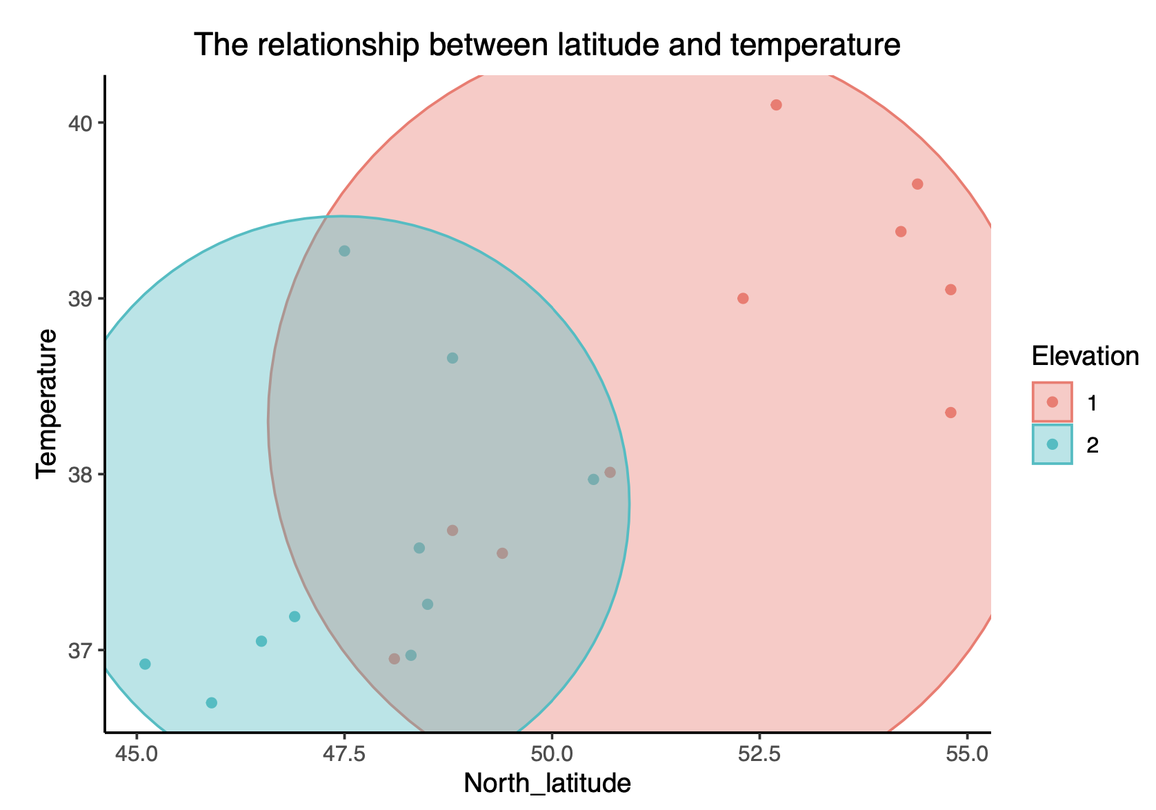
地理位置图
library(ggplot2)
library(viridis)
library(cvTools)
library(dplyr)data <- read.csv("Reef_Check_with_cortad_variables_with_annual_rate_of_SST_change.csv")world_map <- map_data("world")
ggplot() + geom_polygon(data =world_map, aes(x=long, y = lat, group = group), fill="grey", alpha=0.3) +geom_point(data =data, alpha = 0.2, aes(y=Latitude.Degrees, x= Longitude.Degrees , size=Average_bleaching, color=Average_bleaching))  + scale_colour_viridis() + theme_minimal()
igraph网络图
library(igraph)webforum_graph <- webforum[webforum$Date > as.Date("2010-12-01"), ]
webforum_graph <- webforum_graph[webforum_graph$Date < as.Date("2010-12-31"), ]# generate node dataframe
AuthorID <- unique(as.numeric(webforum_graph$AuthorID))
ThreadID <- unique(as.numeric(webforum_graph$ThreadID))
name <- c(AuthorID, ThreadID)
type <- c(rep("Author", length(AuthorID)) , rep("Thread", length(ThreadID)))
webforum_node <- data.frame(name = name, type = type)# generate edge dataframe
webforum_graph <- webforum_graph[,c("AuthorID", "ThreadID")]# generate graph dataframe
graph <- graph_from_data_frame(webforum_graph, directed = FALSE, vertices=webforum_node) set.seed(30208289)plot(graph, layout= layout.fruchterman.reingold, vertex.size=10, vertex.shape="circle", vertex.color=ifelse(V(graph)$type == "Thread", "red", "blue"),vertex.label=NULL, vertex.label.cex=0.7, vertex.label.color='black', vertex.label.dist=0,edge.arrow.size=0.2, edge.width = 0.5, edge.label=V(graph)$year, edge.label.cex=0.5,edge.color="black") 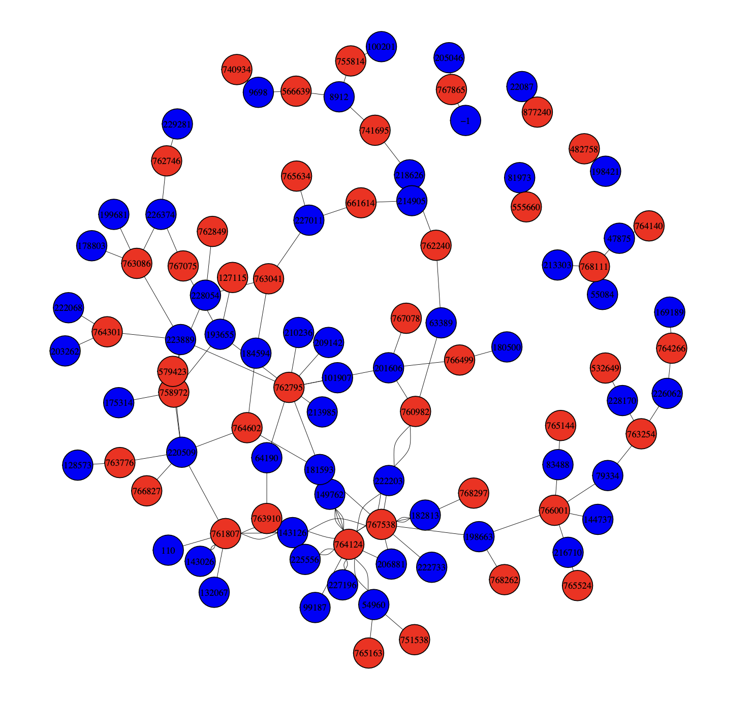
相关文章:
R_handbook_作图专题
ggplot基本作图 1 条形图 library(ggplot2) ggplot(biopics) geom_histogram(aes(x year_release),binwidth1,fill"gray") 2 堆砌柱状图 ggplot(biopics, aes(xyear_release)) geom_bar(aes(fillsubject_sex)) 3 堆砌比例柱状图 ggplot(biopics, aes(xyear_rele…...

关于Python里xlwings库对Excel表格的操作(二十五)
这篇小笔记主要记录如何【如何使用xlwings库的“Chart”类创建一个新图表】。 前面的小笔记已整理成目录,可点链接去目录寻找所需更方便。 【目录部分内容如下】【点击此处可进入目录】 (1)如何安装导入xlwings库; (2…...

2024 年软件工程将如何发展
软件开发目前正在经历一场深刻的变革,其特点是先进自动化的悄然但显着的激增。这一即将发生的转变有望以前所未有的规模简化高质量应用程序的创建和部署。 它不是单一技术引领这一演变,而是创新的融合。从人工智能(AI) 和数字孪生技术,到植根…...

【Git】git基础
Git 命令 git config --globle user.name ""git config --globle user.email ""git config -lgit config --globle --unset []git add []git commit -m ""]git log//当行且美观 git log --prettyoneline//以图形化和简短的方式 git log --grap…...
Linux中账号和权限管理
目录 一.用户账号和组账号: 1.用户账号类型: 2.组账号类型: 3.系统区别用户的方法 : 4.用户账号文件: 二.Linux中账户相关命令: 1.useradd: 2.passwd: 3.usermod:…...
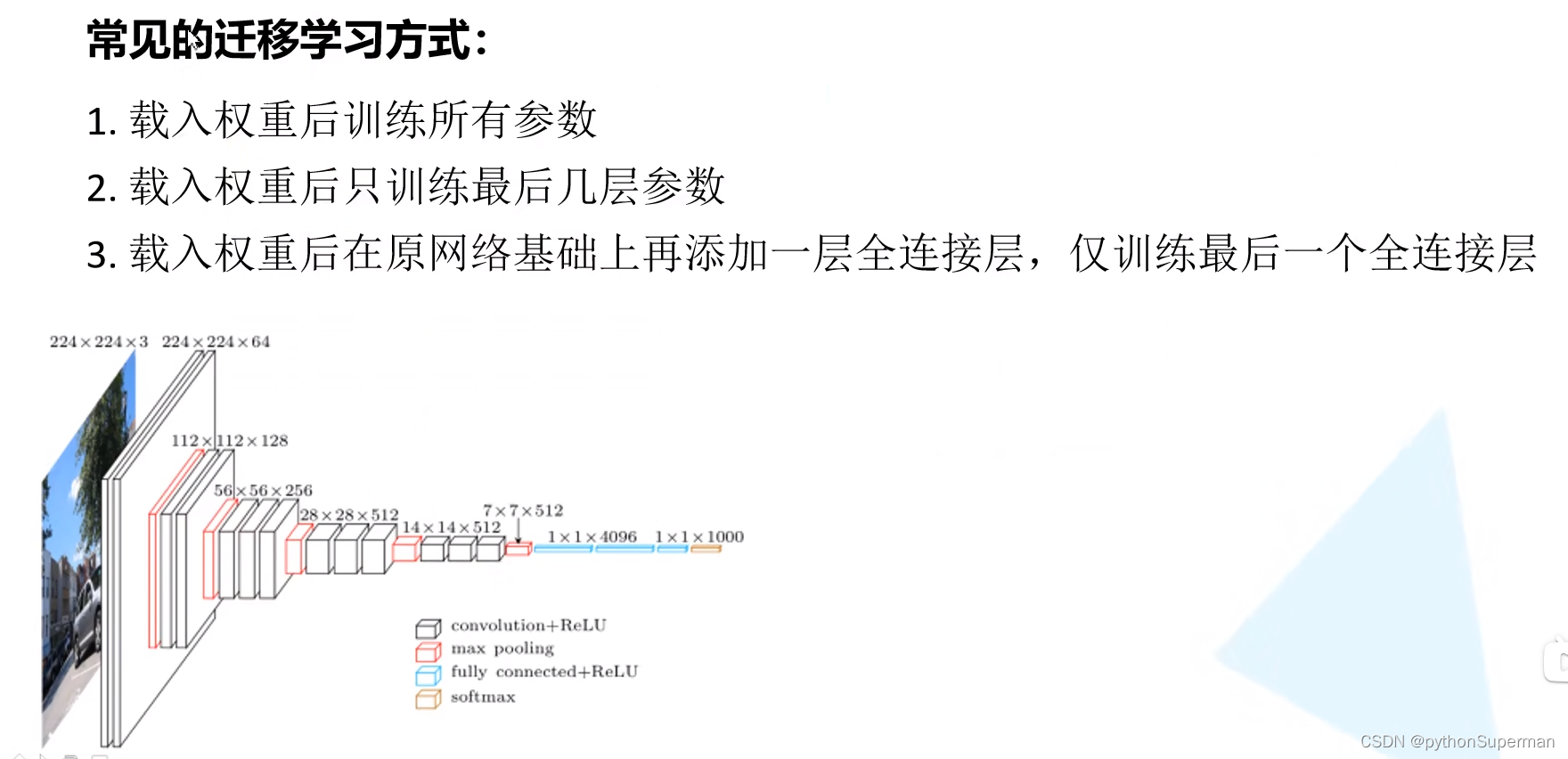
Resnet BatchNormalization 迁移学习
时间:2015 网络中的亮点: 超深的网络结构(突破1000层)提出residual模块使用Batch Normalization加速训练(丢弃dropout) 层数越深效果越好? 是什么样的原因导致更深的网络导致的训练效果更差呢…...

Unity检测地面坡度丨人物上坡检测
Unity检测地面坡度 前言使用 代码 前言 此功能为,人物在爬坡等功能时可以检测地面坡度从而完成向某个方向给力或者完成其他操作 使用 其中我们创建了脚本GradeCalculation,把脚本挂载到人物上即可,或者有其他的使用方式,可自行…...
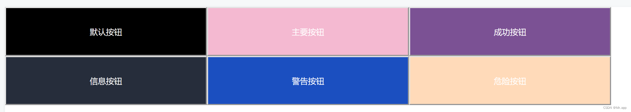
SASS循环
<template><div><button class"btn type-1">默认按钮</button><button class"type-2">主要按钮</button><button class"type-3">成功按钮</button><button class"type-4">信息…...
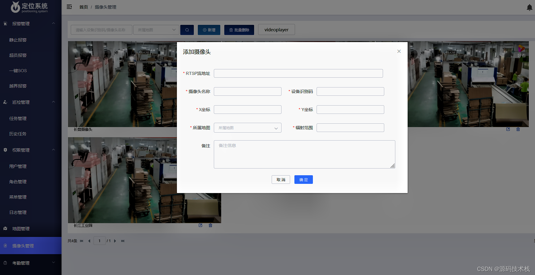
Java超高精度无线定位技术--UWB (超宽带)人员定位系统源码
UWB室内定位技术是一种全新的、与传统通信技术有极大差异的通信新技术。它不需要使用传统通信体制中的载波,而是通过发送和接收具有纳秒或纳秒级以下的极窄脉冲来传输数据,从而具有GHz量级的带宽。 UWB(超宽带)高精度定位系统是一…...

系列十一、解压文件到指定目录
一、解压文件到指定目录 1.1、需求 Linux的/opt目录有一个文件zookeeper-3.4.11.tar.gz,我现在想把该文件解压至/usr/local/目录,那么应该怎么做呢? 语法:tar -zxvf xxx -C /usr/local/ tar -zxvf zookeeper-3.4.11.tar.gz -C /u…...

PHP Swoole Client
PHP常用socket创建TCP连接,使用CURL创建HTTP连接,为了简化操作,Swoole提供了Client类用于实现客户端功能,并增加了异步非阻塞模式,让用户在客户端也能使用事件循环。 作为客户端使用,Swoole Client可以在F…...

《QDebug 2023年12月》
一、Qt Widgets 问题交流 1. 二、Qt Quick 问题交流 1.Q_REVISION 标记的信号槽或者 REVISION 标记的属性,在子类中访问 Q_REVISION 是 Qt 用来做版本控制的一个宏。以 QQuickWindow 为例,继承后去访问 REVISION 标记的 opacity 属性或者 Q_REVISION…...
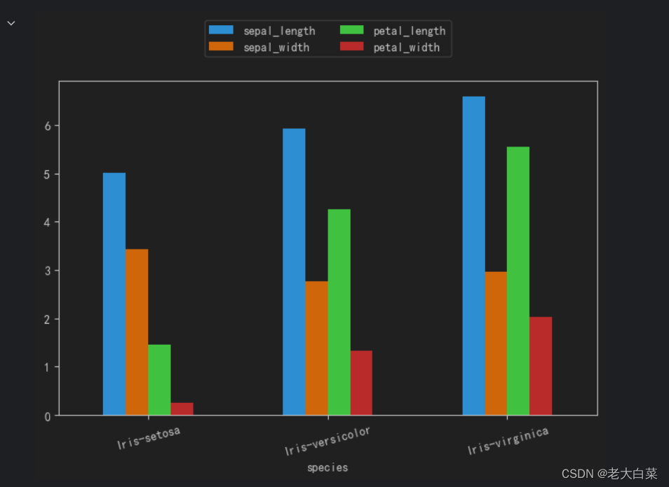
sklearn 中matplotlib编制图表
代码 # 导入pandas库,并为其设置别名pd import pandas as pd import matplotlib.pyplot as plt# 使用pandas的read_csv函数读取名为iris.csv的文件,将数据存储在iris_data变量中 iris_data pd.read_csv(data/iris.txt,sep\t)# 使用groupby方法按照&quo…...
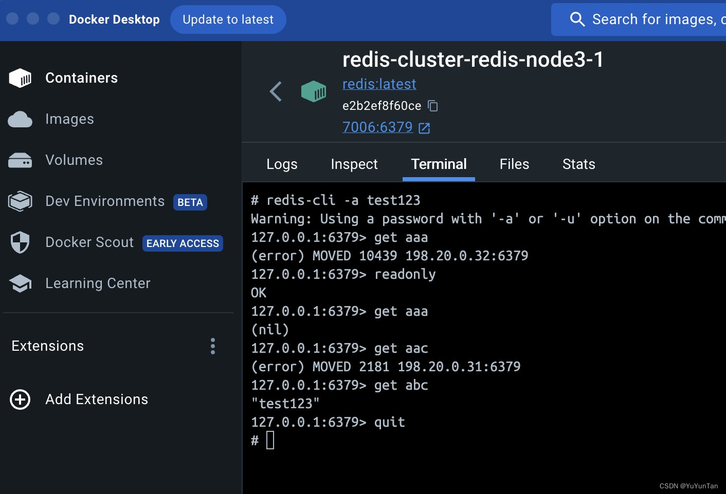
【Docker-Dev】Mac M2 搭建docker的redis环境
Redis的dev环境docker搭建 1、前言2、官方文档重点信息提取2.1、创建redis实例2.2、使用自己的redis.conf文件。 3、单机版redis搭建4、redis集群版4.1、一些验证4.2、一些问题 结语 1、前言 本文主要针对M2下,相应进行开发环境搭建,然后做一个文档记录…...
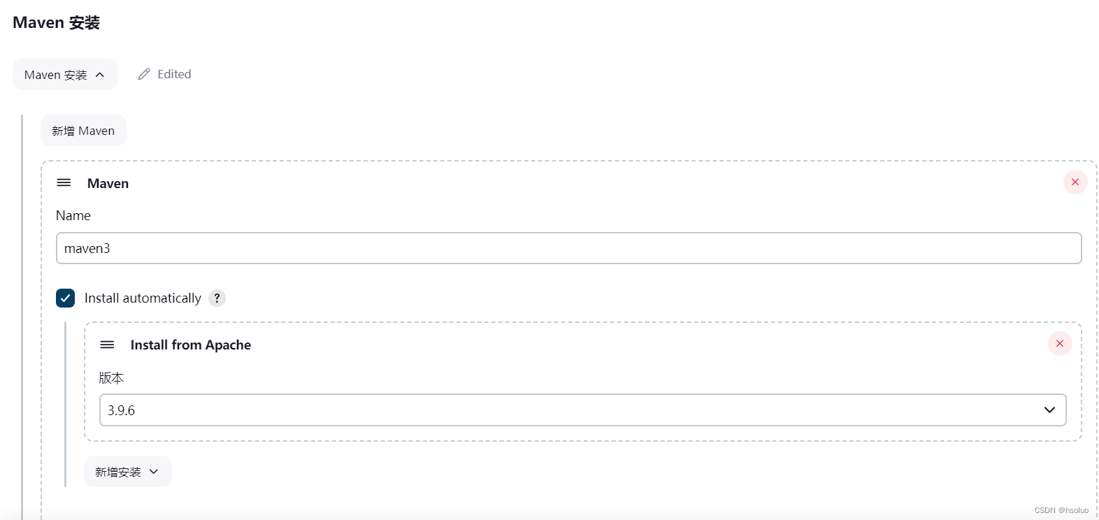
docker +gitee+ jenkins +maven项目 (一)
jenkins环境和插件配置 文章目录 jenkins环境和插件配置前言一、环境版本二、jenkins插件三、环境安装总结 前言 现在基本都是走自动化运维,想到用docker 来部署jenkins ,然后jenkins来部署java代码,做到了开箱即用,自动发布代码…...
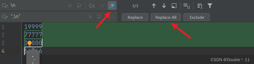
IDEA 开发中常用的快捷键
目录 Ctrl 的快捷键 Alt 的快捷键 Shift 的快捷键 Ctrl Alt 的快捷键 Ctrl Shift 的快捷键 其他的快捷键 Ctrl 的快捷键 Ctrl F 在当前文件进行文本查找 (必备) Ctrl R 在当前文件进行文本替换 (必备) Ctrl Z 撤…...

Ubuntu Desktop 死机处理
Ubuntu Desktop 死机处理 当 Ubuntu Desktop 死机时,除了长按电源键重启,还可以使用如下两种方式处理。 方式1:ctrlaltFn 使用 ctrl alt F3~F6: 切换到其他 tty 命令行。 执行 top 命令查看资源占用最多的进程,然后使用 kill…...

Hermite矩阵
Hermite矩阵 文章目录 Hermite矩阵一、正规矩阵【定义】A^H^矩阵【定理】 A^H^的运算性质【定义】正规矩阵、特殊的正规矩阵【定理】与正规矩阵酉相似的矩阵也是正规矩阵【定理】正规的上(下)三角矩阵必为对角矩阵【定义】复向量的内积【定理】Schmitt正交化 二、酉矩阵&#x…...
)
HTML 实操试题(二)
创建一个简单的HTML文档: 包含<!DOCTYPE html>声明。包含<html>标签,并设置lang属性为英语。包含<head>标签,其中包含<meta charset"UTF-8">和一个自定义的页面标题。包含<body>标签,其…...
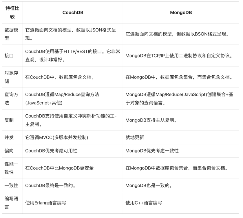
MongoDB 面试题
MongoDB 面试题 1. 什么是MongoDB? MongoDB是一种非关系型数据库,被广泛用于大型数据存储和分布式系统的构建。MongoDB支持的数据模型比传统的关系型数据库更加灵活,支持动态查询和索引,也支持BSON格式的数据存储,这…...
测试微信模版消息推送
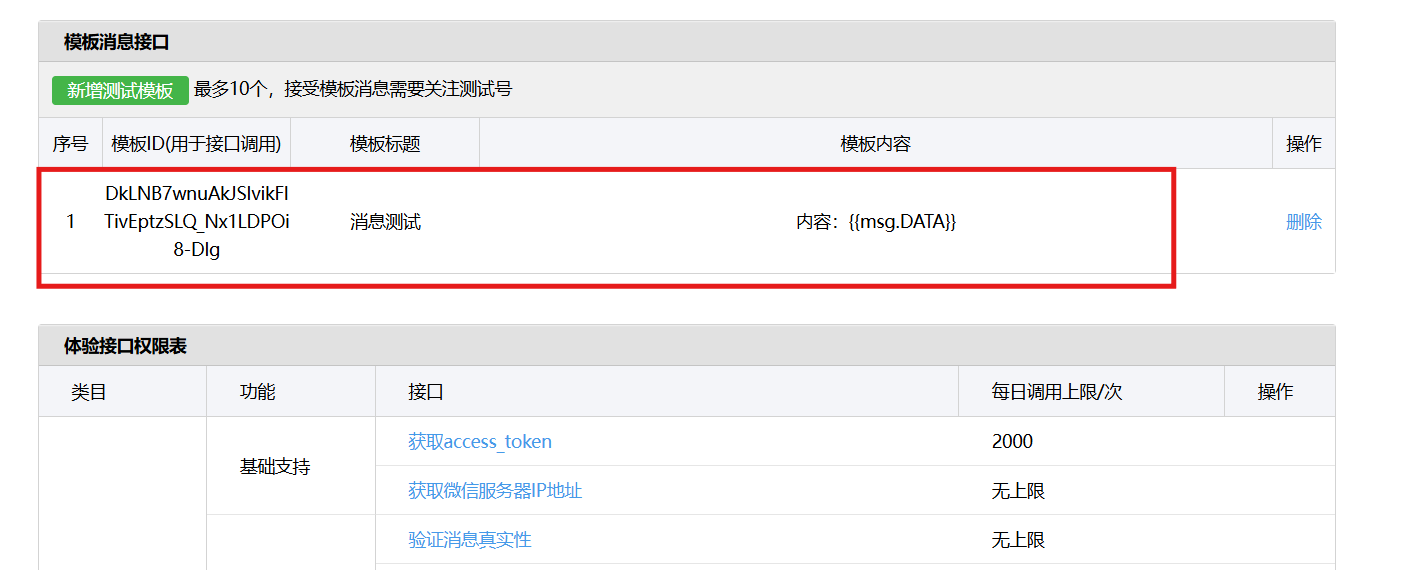
进入“开发接口管理”--“公众平台测试账号”,无需申请公众账号、可在测试账号中体验并测试微信公众平台所有高级接口。 获取access_token: 自定义模版消息: 关注测试号:扫二维码关注测试号。 发送模版消息: import requests da…...

C++初阶-list的底层
目录 1.std::list实现的所有代码 2.list的简单介绍 2.1实现list的类 2.2_list_iterator的实现 2.2.1_list_iterator实现的原因和好处 2.2.2_list_iterator实现 2.3_list_node的实现 2.3.1. 避免递归的模板依赖 2.3.2. 内存布局一致性 2.3.3. 类型安全的替代方案 2.3.…...
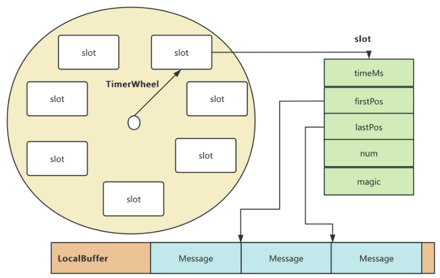
RocketMQ延迟消息机制
两种延迟消息 RocketMQ中提供了两种延迟消息机制 指定固定的延迟级别 通过在Message中设定一个MessageDelayLevel参数,对应18个预设的延迟级别指定时间点的延迟级别 通过在Message中设定一个DeliverTimeMS指定一个Long类型表示的具体时间点。到了时间点后…...
使用rpicam-app通过网络流式传输视频)
树莓派超全系列教程文档--(62)使用rpicam-app通过网络流式传输视频
使用rpicam-app通过网络流式传输视频 使用 rpicam-app 通过网络流式传输视频UDPTCPRTSPlibavGStreamerRTPlibcamerasrc GStreamer 元素 文章来源: http://raspberry.dns8844.cn/documentation 原文网址 使用 rpicam-app 通过网络流式传输视频 本节介绍来自 rpica…...

微软PowerBI考试 PL300-选择 Power BI 模型框架【附练习数据】
微软PowerBI考试 PL300-选择 Power BI 模型框架 20 多年来,Microsoft 持续对企业商业智能 (BI) 进行大量投资。 Azure Analysis Services (AAS) 和 SQL Server Analysis Services (SSAS) 基于无数企业使用的成熟的 BI 数据建模技术。 同样的技术也是 Power BI 数据…...
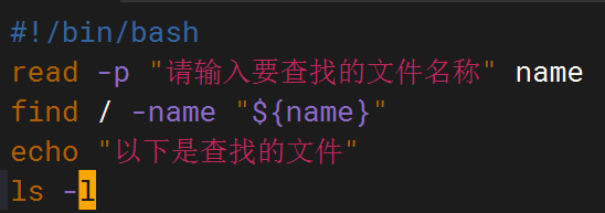
shell脚本--常见案例
1、自动备份文件或目录 2、批量重命名文件 3、查找并删除指定名称的文件: 4、批量删除文件 5、查找并替换文件内容 6、批量创建文件 7、创建文件夹并移动文件 8、在文件夹中查找文件...

前端倒计时误差!
提示:记录工作中遇到的需求及解决办法 文章目录 前言一、误差从何而来?二、五大解决方案1. 动态校准法(基础版)2. Web Worker 计时3. 服务器时间同步4. Performance API 高精度计时5. 页面可见性API优化三、生产环境最佳实践四、终极解决方案架构前言 前几天听说公司某个项…...

Android Bitmap治理全解析:从加载优化到泄漏防控的全生命周期管理
引言 Bitmap(位图)是Android应用内存占用的“头号杀手”。一张1080P(1920x1080)的图片以ARGB_8888格式加载时,内存占用高达8MB(192010804字节)。据统计,超过60%的应用OOM崩溃与Bitm…...
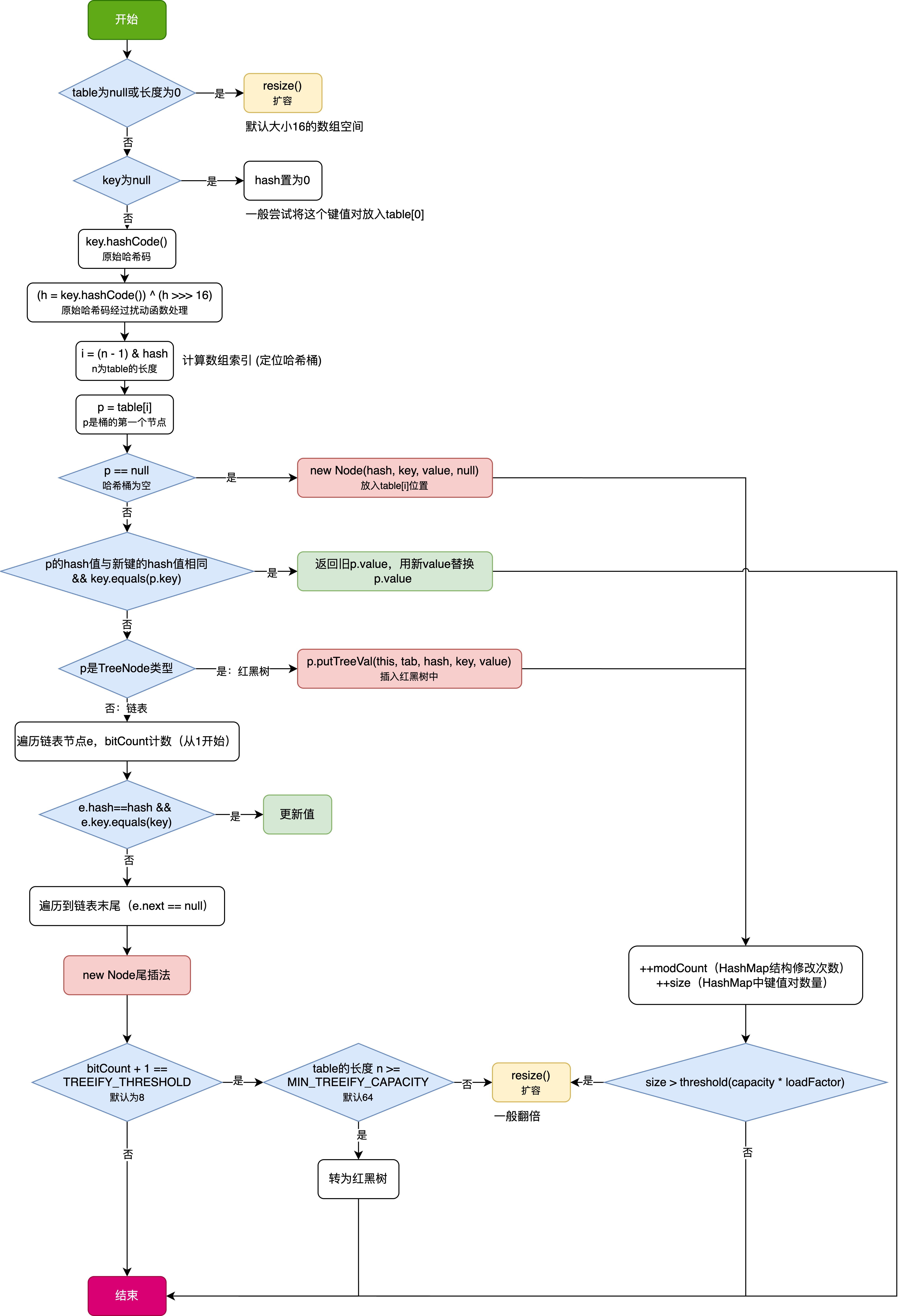
HashMap中的put方法执行流程(流程图)
1 put操作整体流程 HashMap 的 put 操作是其最核心的功能之一。在 JDK 1.8 及以后版本中,其主要逻辑封装在 putVal 这个内部方法中。整个过程大致如下: 初始判断与哈希计算: 首先,putVal 方法会检查当前的 table(也就…...
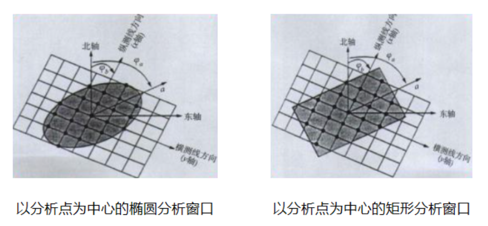
论文笔记——相干体技术在裂缝预测中的应用研究
目录 相关地震知识补充地震数据的认识地震几何属性 相干体算法定义基本原理第一代相干体技术:基于互相关的相干体技术(Correlation)第二代相干体技术:基于相似的相干体技术(Semblance)基于多道相似的相干体…...