PyTorch搭建Autoformer实现长序列时间序列预测
目录
- I. 前言
- II. Autoformer
- III. 代码
- 3.1 Encoder输入
- 3.1.1 Token Embedding
- 3.1.2 Temporal Embedding
- 3.2 Decoder输入
- 3.3 Encoder与Decoder
- 3.3.1 初始化
- 3.3.2 Encoder
- 3.3.3 Decoder
- IV. 实验
I. 前言
前面已经写了很多关于时间序列预测的文章:
- 深入理解PyTorch中LSTM的输入和输出(从input输入到Linear输出)
- PyTorch搭建LSTM实现时间序列预测(负荷预测)
- PyTorch中利用LSTMCell搭建多层LSTM实现时间序列预测
- PyTorch搭建LSTM实现多变量时间序列预测(负荷预测)
- PyTorch搭建双向LSTM实现时间序列预测(负荷预测)
- PyTorch搭建LSTM实现多变量多步长时间序列预测(一):直接多输出
- PyTorch搭建LSTM实现多变量多步长时间序列预测(二):单步滚动预测
- PyTorch搭建LSTM实现多变量多步长时间序列预测(三):多模型单步预测
- PyTorch搭建LSTM实现多变量多步长时间序列预测(四):多模型滚动预测
- PyTorch搭建LSTM实现多变量多步长时间序列预测(五):seq2seq
- PyTorch中实现LSTM多步长时间序列预测的几种方法总结(负荷预测)
- PyTorch-LSTM时间序列预测中如何预测真正的未来值
- PyTorch搭建LSTM实现多变量输入多变量输出时间序列预测(多任务学习)
- PyTorch搭建ANN实现时间序列预测(风速预测)
- PyTorch搭建CNN实现时间序列预测(风速预测)
- PyTorch搭建CNN-LSTM混合模型实现多变量多步长时间序列预测(负荷预测)
- PyTorch搭建Transformer实现多变量多步长时间序列预测(负荷预测)
- PyTorch时间序列预测系列文章总结(代码使用方法)
- TensorFlow搭建LSTM实现时间序列预测(负荷预测)
- TensorFlow搭建LSTM实现多变量时间序列预测(负荷预测)
- TensorFlow搭建双向LSTM实现时间序列预测(负荷预测)
- TensorFlow搭建LSTM实现多变量多步长时间序列预测(一):直接多输出
- TensorFlow搭建LSTM实现多变量多步长时间序列预测(二):单步滚动预测
- TensorFlow搭建LSTM实现多变量多步长时间序列预测(三):多模型单步预测
- TensorFlow搭建LSTM实现多变量多步长时间序列预测(四):多模型滚动预测
- TensorFlow搭建LSTM实现多变量多步长时间序列预测(五):seq2seq
- TensorFlow搭建LSTM实现多变量输入多变量输出时间序列预测(多任务学习)
- TensorFlow搭建ANN实现时间序列预测(风速预测)
- TensorFlow搭建CNN实现时间序列预测(风速预测)
- TensorFlow搭建CNN-LSTM混合模型实现多变量多步长时间序列预测(负荷预测)
- PyG搭建图神经网络实现多变量输入多变量输出时间序列预测
- PyTorch搭建GNN-LSTM和LSTM-GNN模型实现多变量输入多变量输出时间序列预测
- PyG Temporal搭建STGCN实现多变量输入多变量输出时间序列预测
- 时序预测中Attention机制是否真的有效?盘点LSTM/RNN中24种Attention机制+效果对比
- 详解Transformer在时序预测中的Encoder和Decoder过程:以负荷预测为例
- (PyTorch)TCN和RNN/LSTM/GRU结合实现时间序列预测
- PyTorch搭建Informer实现长序列时间序列预测
- PyTorch搭建Autoformer实现长序列时间序列预测
上一篇文章讲了长序列时间序列预测的第一个模型Informer,Informer发表于AAAI 2021。这一篇文章讲第二个长序列时间预测模型Autoformer,Autoformer为NeurIPS 2021中《Autoformer: Decomposition Transformers with Auto-Correlation for Long-Term Series Forecasting》提出的模型,比Informer晚了差不多半年。
II. Autoformer
Autoformer的目的是待预测的长度远大于输入长度的长期序列预测问题,即就有有限的信息预测更长远的未来。
Autoformer的创新点如下:
- 长序列中的复杂时间模式使得Transformer中的注意力机制难以发现可靠的时序依赖。因此,Autoformer提出将时间序列分解嵌入到深度学习模型中,在这之前,分解一般都是用作数据预处理,如EMD分解等。可学习的分解可以帮助模型从复杂的序列数据中分解出可预测性更强的组分。
- Transformer的时间复杂度较高,造成了信息利用的瓶颈。因此,Autoformer中基于随机过程理论,提出了Auto-correlation机制来代替了Transformer中的基于point-wise的self-attention机制,实现序列级(series-wise)连接和 O ( L log L ) O(L \log L) O(LlogL)的时间复杂度,打破信息利用瓶颈。
更具体的原理就不做讲解了,网上已经有了很多类似的文章,这篇文章主要讲解代码的使用,重点是如何对作者公开的源代码进行改动,以更好地适配大多数人自身的数据,使得读者只需要改变少数几个参数就能实现数据集的更换。
III. 代码
3.1 Encoder输入
传统Transformer中在编码阶段需要进行的第一步就是在原始序列的基础上添加位置编码,而在Autoformer中,输入由2部分组成,即Token Embedding和Temporal Embedding,没有位置编码。
我们假设输入的序列长度为(batch_size, seq_len, enc_in),如果用过去96个时刻的所有13个变量预测未来时刻的值,那么输入即为(batch_size, 96, 13)。
3.1.1 Token Embedding
Autoformer输入的第1部分是对原始输入进行编码,本质是利用一个1维卷积对原始序列进行特征提取,并且序列的维度从原始的enc_in变换到d_model,代码如下:
class TokenEmbedding(nn.Module):def __init__(self, c_in, d_model):super(TokenEmbedding, self).__init__()padding = 1 if torch.__version__ >= '1.5.0' else 2self.tokenConv = nn.Conv1d(in_channels=c_in, out_channels=d_model,kernel_size=3, padding=padding, padding_mode='circular')for m in self.modules():if isinstance(m, nn.Conv1d):nn.init.kaiming_normal_(m.weight, mode='fan_in', nonlinearity='leaky_relu')def forward(self, x):x = self.tokenConv(x.permute(0, 2, 1)).transpose(1, 2)return x
输入x的大小为(batch_size, seq_len, enc_in),需要先将后两个维度交换以适配1维卷积,接着让数据通过tokenConv,由于添加了padding,因此经过后seq_len维度不改变,经过TokenEmbedding后得到大小为(batch_size, seq_len, d_model)的输出。
3.1.2 Temporal Embedding
Autoformer输入的第2部分是对时间戳进行编码,即年月日星期时分秒等进行编码。这一部分与Informer中一致,使用了两种编码方式,我们依次解析。第一种编码方式TemporalEmbedding代码如下:
class TemporalEmbedding(nn.Module):def __init__(self, d_model, embed_type='fixed', freq='h'):super(TemporalEmbedding, self).__init__()minute_size = 4hour_size = 24weekday_size = 7day_size = 32month_size = 13Embed = FixedEmbedding if embed_type == 'fixed' else nn.Embeddingif freq == 't':self.minute_embed = Embed(minute_size, d_model)self.hour_embed = Embed(hour_size, d_model)self.weekday_embed = Embed(weekday_size, d_model)self.day_embed = Embed(day_size, d_model)self.month_embed = Embed(month_size, d_model)def forward(self, x):x = x.long()minute_x = self.minute_embed(x[:, :, 4]) if hasattr(self, 'minute_embed') else 0.hour_x = self.hour_embed(x[:, :, 3])weekday_x = self.weekday_embed(x[:, :, 2])day_x = self.day_embed(x[:, :, 1])month_x = self.month_embed(x[:, :, 0])return hour_x + weekday_x + day_x + month_x + minute_x
TemporalEmbedding的输入要求是(batch_size, seq_len, 5),5表示每个时间戳的月、天、星期(星期一到星期七)、小时以及刻钟数(一刻钟15分钟)。代码中对五个值分别进行了编码,编码方式有两种,一种是FixedEmbedding,它使用位置编码作为embedding的参数,不需要训练参数;另一种就是torch自带的nn.Embedding,参数是可训练的。
更具体的,作者将月、天、星期、小时以及刻钟的范围分别限制在了13、32、7、24以及4。即保证输入每个时间戳的月份数都在0-12,天数都在0-31,星期都在0-6,小时数都在0-23,刻钟数都在0-3。例如2024/04/05/12:13,星期五,输入应该是(4, 5, 5, 13, 0)。注意12:13小时数应该为13,小于等于12:00但大于11:00如11:30才为12。
对时间戳进行编码的第二种方式为TimeFeatureEmbedding:
class TimeFeatureEmbedding(nn.Module):def __init__(self, d_model, embed_type='timeF', freq='h'):super(TimeFeatureEmbedding, self).__init__()freq_map = {'h': 4, 't': 5, 's': 6, 'm': 1, 'a': 1, 'w': 2, 'd': 3, 'b': 3}d_inp = freq_map[freq]self.embed = nn.Linear(d_inp, d_model)def forward(self, x):return self.embed(x)
TimeFeatureEmbedding的输入为(batch_size, seq_len, d_inp),d_inp有多达8种选择。具体来说针对时间戳2024/04/05/12:13,以freq='h’为例,其输入应该是(月份、日期、星期、小时),即(4, 5, 5, 13),然后针对输入通过以下函数将所有数据转换到-0.5到0.5之间:
def time_features(dates, timeenc=1, freq='h'):"""> `time_features` takes in a `dates` dataframe with a 'dates' column and extracts the date down to `freq` where freq can be any of the following if `timeenc` is 0: > * m - [month]> * w - [month]> * d - [month, day, weekday]> * b - [month, day, weekday]> * h - [month, day, weekday, hour]> * t - [month, day, weekday, hour, *minute]> > If `timeenc` is 1, a similar, but different list of `freq` values are supported (all encoded between [-0.5 and 0.5]): > * Q - [month]> * M - [month]> * W - [Day of month, week of year]> * D - [Day of week, day of month, day of year]> * B - [Day of week, day of month, day of year]> * H - [Hour of day, day of week, day of month, day of year]> * T - [Minute of hour*, hour of day, day of week, day of month, day of year]> * S - [Second of minute, minute of hour, hour of day, day of week, day of month, day of year]*minute returns a number from 0-3 corresponding to the 15 minute period it falls into."""if timeenc == 0:dates['month'] = dates.date.apply(lambda row: row.month, 1)dates['day'] = dates.date.apply(lambda row: row.day, 1)dates['weekday'] = dates.date.apply(lambda row: row.weekday(), 1)dates['hour'] = dates.date.apply(lambda row: row.hour, 1)dates['minute'] = dates.date.apply(lambda row: row.minute, 1)dates['minute'] = dates.minute.map(lambda x: x // 15)freq_map = {'y': [], 'm': ['month'], 'w': ['month'], 'd': ['month', 'day', 'weekday'],'b': ['month', 'day', 'weekday'], 'h': ['month', 'day', 'weekday', 'hour'],'t': ['month', 'day', 'weekday', 'hour', 'minute'],}return dates[freq_map[freq.lower()]].valuesif timeenc == 1:dates = pd.to_datetime(dates.date.values)return np.vstack([feat(dates) for feat in time_features_from_frequency_str(freq)]).transpose(1, 0)
当freq为’t’时,输入应该为[‘month’, ‘day’, ‘weekday’, ‘hour’, ‘minute’],其他类似。当通过上述函数将四个数转换为-0.5到0.5之间后,再利用TimeFeatureEmbedding中的self.embed = nn.Linear(d_inp, d_model)来将维度从4转换到d_model,因此最终返回的输出大小也为(batch_size, seq_len, d_model)。
最终,代码中通过一个DataEmbedding_wo_pos类来将2种编码放在一起:
class DataEmbedding_wo_pos(nn.Module):def __init__(self, c_in, d_model, embed_type='fixed', freq='h', dropout=0.1):super(DataEmbedding_wo_pos, self).__init__()self.value_embedding = TokenEmbedding(c_in=c_in, d_model=d_model)self.position_embedding = PositionalEmbedding(d_model=d_model)self.temporal_embedding = TemporalEmbedding(d_model=d_model, embed_type=embed_type,freq=freq) if embed_type != 'timeF' else TimeFeatureEmbedding(d_model=d_model, embed_type=embed_type, freq=freq)self.dropout = nn.Dropout(p=dropout)def forward(self, x, x_mark):x = self.value_embedding(x) + self.temporal_embedding(x_mark)return self.dropout(x)
3.2 Decoder输入
在Informer中,编码器和解码器的输入大同小异,都由三部分组成,而在Autoformer中,二者存在差别。
在解码器中,进行Token Embedding的不是原始的时间序列,而是seasonal part,这部分在3.3节中进行讲解。
3.3 Encoder与Decoder
完整的Autoformer代码如下:
class Autoformer(nn.Module):"""Autoformer is the first method to achieve the series-wise connection,with inherent O(LlogL) complexity"""def __init__(self, args):super(Autoformer, self).__init__()self.seq_len = args.seq_lenself.label_len = args.label_lenself.pred_len = args.pred_lenself.output_attention = args.output_attention# Decompkernel_size = args.moving_avgself.decomp = series_decomp(kernel_size)# Embedding# The series-wise connection inherently contains the sequential information.# Thus, we can discard the position embedding of transformers.self.enc_embedding = DataEmbedding_wo_pos(args.enc_in, args.d_model, args.embed, args.freq,args.dropout)self.dec_embedding = DataEmbedding_wo_pos(args.dec_in, args.d_model, args.embed, args.freq,args.dropout)# Encoderself.encoder = Encoder([EncoderLayer(AutoCorrelationLayer(AutoCorrelation(False, args.factor, attention_dropout=args.dropout,output_attention=args.output_attention),args.d_model, args.n_heads),args.d_model,args.d_ff,moving_avg=args.moving_avg,dropout=args.dropout,activation=args.activation) for l in range(args.e_layers)],norm_layer=my_Layernorm(args.d_model))# Decoderself.decoder = Decoder([DecoderLayer(AutoCorrelationLayer(AutoCorrelation(True, args.factor, attention_dropout=args.dropout,output_attention=False),args.d_model, args.n_heads),AutoCorrelationLayer(AutoCorrelation(False, args.factor, attention_dropout=args.dropout,output_attention=False),args.d_model, args.n_heads),args.d_model,args.c_out,args.d_ff,moving_avg=args.moving_avg,dropout=args.dropout,activation=args.activation,)for l in range(args.d_layers)],norm_layer=my_Layernorm(args.d_model),projection=nn.Linear(args.d_model, args.c_out, bias=True))def forward(self, x_enc, x_mark_enc, x_dec, x_mark_dec,enc_self_mask=None, dec_self_mask=None, dec_enc_mask=None):# decomp initmean = torch.mean(x_enc, dim=1).unsqueeze(1).repeat(1, self.pred_len, 1)zeros = torch.zeros([x_dec.shape[0], self.pred_len, x_dec.shape[2]], device=x_enc.device)seasonal_init, trend_init = self.decomp(x_enc)# decoder inputtrend_init = torch.cat([trend_init[:, -self.label_len:, :], mean], dim=1)seasonal_init = torch.cat([seasonal_init[:, -self.label_len:, :], zeros], dim=1)# encenc_out = self.enc_embedding(x_enc, x_mark_enc)enc_out, attns = self.encoder(enc_out, attn_mask=enc_self_mask)# decdec_out = self.dec_embedding(seasonal_init, x_mark_dec)seasonal_part, trend_part = self.decoder(dec_out, enc_out, x_mask=dec_self_mask, cross_mask=dec_enc_mask,trend=trend_init)# finaldec_out = trend_part + seasonal_partif self.output_attention:return dec_out[:, -self.pred_len:, :], attnselse:return dec_out[:, -self.pred_len:, :] # [B, L, D]
观察forward,主要的输入为x_enc, x_mark_enc, x_dec, x_mark_dec,下边依次介绍:
- x_enc: 编码器输入,大小为
(batch_size, seq_len, enc_in),在这篇文章中,我们使用前96个时刻的所有13个变量预测未来24个时刻的所有13个变量,所以这里x_enc的输入应该是(batch_size, 96, 13)。 - x_mark_enc:编码器的时间戳输入,大小分情况,本文中采用频率freq='h’的TimeFeatureEmbedding编码方式,所以应该输入[‘month’, ‘day’, ‘weekday’, ‘hour’],大小为
(batch_size, 96, 4)。 - x_dec,解码器输入,大小为
(batch_size, label_len+pred_len, dec_in),其中dec_in为解码器输入的变量个数,也为13。在Informer中,为了避免step-by-step的解码结构,作者直接将x_enc中后label_len个时刻的数据和要预测时刻的数据进行拼接得到解码器输入。在本次实验中,由于需要预测未来24个时刻的数据,所以pred_len=24,向前看48个时刻,所以label_len=48,最终解码器的输入维度应该为(batch_size, 48+24=72, 13)。 - x_mark_dec,解码器的时间戳输入,大小为
(batch_size, 72, 4)。
为了方便理解编码器和解码器的输入,给一个具体的例子:假设某个样本编码器的输入为1-96时刻的所有13个变量,即x_enc大小为(96, 13),x_mark_enc大小为(96, 4),表示每个时刻的[‘month’, ‘day’, ‘weekday’, ‘hour’];解码器输入为编码器输入的后label_len=48+要预测的pred_len=24个时刻的数据,即49-120时刻的所有13个变量,x_dec大小为(72, 13),同理x_mark_dec大小为(72, 4)。
为了防止数据泄露,在预测97-120时刻的数据时,解码器输入x_dec中不能包含97-120时刻的真实数据,在原文中,作者用24个0来代替,代码如下:
dec_inp = torch.zeros_like(batch_y[:, -self.args.pred_len:, :]).float()
dec_inp = torch.cat([batch_y[:, :self.args.label_len, :], dec_inp], dim=1).float().to(self.device)
3.3.1 初始化
这部分代码如下:
# decomp init
mean = torch.mean(x_enc, dim=1).unsqueeze(1).repeat(1, self.pred_len, 1)
zeros = torch.zeros([x_dec.shape[0], self.pred_len, x_dec.shape[2]], device=x_enc.device)
seasonal_init, trend_init = self.decomp(x_enc)
# decoder input
trend_init = torch.cat([trend_init[:, -self.label_len:, :], mean], dim=1)
seasonal_init = torch.cat([seasonal_init[:, -self.label_len:, :], zeros], dim=1)
首先是:
mean = torch.mean(x_enc, dim=1).unsqueeze(1).repeat(1, self.pred_len, 1)
这一句代码首先将大小为(batch_size, 96, 13)的x_enc沿着seq_len维度求平均,然后再repeat变成(batch_size, 24, 13),其中24表示pred_len,13表示96个时刻在13个变量上的平均值。
接着初始化大小为(batch_size, 24, 13)的全0矩阵zeros。
接着对x_enc进行分解得到两个趋势分量:
seasonal_init, trend_init = self.decomp(x_enc)
更具体来说,首先利用series_decomp模块来对x_enc也就是大小为(batch_size, seq_len=96, enc_in=13)的编码器输入进行分解,series_decomp代码如下所示:
class moving_avg(nn.Module):"""Moving average block to highlight the trend of time series"""def __init__(self, kernel_size, stride):super(moving_avg, self).__init__()self.kernel_size = kernel_sizeself.avg = nn.AvgPool1d(kernel_size=kernel_size, stride=stride, padding=0)def forward(self, x):# padding on the both ends of time seriesfront = x[:, 0:1, :].repeat(1, (self.kernel_size - 1) // 2, 1)end = x[:, -1:, :].repeat(1, (self.kernel_size - 1) // 2, 1)x = torch.cat([front, x, end], dim=1)x = self.avg(x.permute(0, 2, 1))x = x.permute(0, 2, 1)return xclass series_decomp(nn.Module):"""Series decomposition block"""def __init__(self, kernel_size):super(series_decomp, self).__init__()self.moving_avg = moving_avg(kernel_size, stride=1)def forward(self, x):moving_mean = self.moving_avg(x)res = x - moving_meanreturn res, moving_mean
输入的x为x_enc,大小为(batch_size, seq_len=96, enc_in=13),所谓的分解就是先利用一个nn.AvgPool1d来对x_enc进行池化,针对seq_len这个维度进行平均池化,即每kernel_size长度求一次平均。由于添加了padding,所以池化后大小不变,依旧为(batch_size, seq_len, enc_in),池化后的这部分即为初始的季节趋势seasonal_init,x_enc减去seasonal_init即为trend_init,反映短期波动。
最后是处理decoder的初始输入:
# decoder input
trend_init = torch.cat([trend_init[:, -self.label_len:, :], mean], dim=1)
seasonal_init = torch.cat([seasonal_init[:, -self.label_len:, :], zeros], dim=1)
trend_init大小为(batch_size, 96, 13),我们只取其后label_len=48个数据,然后和大小为(batch_size, 24, 13)mean进行拼接,大小变成(batch_size, 48+24=72, 13),即trend_init的前部分为x_enc分解得到,后部分为x_enc中所有时刻的平均值。seasonal_init大小为(batch_size, 96, 13),我们同样只取其后label_len个数据,然后再和0进行拼接得到(batch_size, 48+24=72, 13),即seasonal_init的前部分为x_enc分解得到,后部分为0。
3.3.2 Encoder
Encoder过程如下所示:
enc_out = self.enc_embedding(x_enc, x_mark_enc)
enc_out, attns = self.encoder(enc_out, attn_mask=enc_self_mask)
这部分和上一篇文章讲的Informer类似,区别只是将注意力机制换成了AutoCorrelation,有关AutoCorrelation这里不做详细介绍。
3.3.3 Decoder
Decoder过程如下所示:
# dec
dec_out = self.dec_embedding(seasonal_init, x_mark_dec)
seasonal_part, trend_part = self.decoder(dec_out, enc_out, x_mask=dec_self_mask, cross_mask=dec_enc_mask, trend=trend_init)
# final
dec_out = trend_part + seasonal_part
首先是利用seasonal_init进行Token Embedding编码,而不是Informer中的x_dec,seasonal_init大小和x_dec一致,都为(batch_size, 48+24=72, 13)。
接着是解码过程:
seasonal_part, trend_part = self.decoder(dec_out, enc_out, x_mask=dec_self_mask, cross_mask=dec_enc_mask, trend=trend_init)
self.decoder的详细过程:
class Decoder(nn.Module):"""Autoformer encoder"""def __init__(self, layers, norm_layer=None, projection=None):super(Decoder, self).__init__()self.layers = nn.ModuleList(layers)self.norm = norm_layerself.projection = projectiondef forward(self, x, cross, x_mask=None, cross_mask=None, trend=None):for layer in self.layers:x, residual_trend = layer(x, cross, x_mask=x_mask, cross_mask=cross_mask)trend = trend + residual_trendif self.norm is not None:x = self.norm(x)if self.projection is not None:x = self.projection(x)return x, trend
直接看forward,Decoder中有很多DecoderLayer,每个DecoderLayer要求的输入为x, cross和trend,x即为dec_out,大小为(batch_size, 48+24=72, 13),cross即编码器输出enc_out,大小为(batch_size, seq_len=96, d_model)。trend即为trend_init,大小为(batch_size, 48+24=72, 13),解码器利用dec_out和enc_out做AutoCorrelation得到x和残差:
class DecoderLayer(nn.Module):"""Autoformer decoder layer with the progressive decomposition architecture"""def __init__(self, self_attention, cross_attention, d_model, c_out, d_ff=None,moving_avg=25, dropout=0.1, activation="relu"):super(DecoderLayer, self).__init__()d_ff = d_ff or 4 * d_modelself.self_attention = self_attentionself.cross_attention = cross_attentionself.conv1 = nn.Conv1d(in_channels=d_model, out_channels=d_ff, kernel_size=1, bias=False)self.conv2 = nn.Conv1d(in_channels=d_ff, out_channels=d_model, kernel_size=1, bias=False)self.decomp1 = series_decomp(moving_avg)self.decomp2 = series_decomp(moving_avg)self.decomp3 = series_decomp(moving_avg)self.dropout = nn.Dropout(dropout)self.projection = nn.Conv1d(in_channels=d_model, out_channels=c_out, kernel_size=3, stride=1, padding=1,padding_mode='circular', bias=False)self.activation = F.relu if activation == "relu" else F.geludef forward(self, x, cross, x_mask=None, cross_mask=None):x = x + self.dropout(self.self_attention(x, x, x,attn_mask=x_mask)[0])x, trend1 = self.decomp1(x)x = x + self.dropout(self.cross_attention(x, cross, cross,attn_mask=cross_mask)[0])x, trend2 = self.decomp2(x)y = xy = self.dropout(self.activation(self.conv1(y.transpose(-1, 1))))y = self.dropout(self.conv2(y).transpose(-1, 1))x, trend3 = self.decomp3(x + y)residual_trend = trend1 + trend2 + trend3residual_trend = self.projection(residual_trend.permute(0, 2, 1)).transpose(1, 2)return x, residual_trend
然后将残累加到初始的trend上,多层结束后最终返回x和trend。
finally,作者将x和trend相加得到解码器的最终输出:
dec_out = trend_part + seasonal_part
dec_out大小依旧为(batch_size, 48+24=72, 13),后pred_len=24个即为预测值:
if self.output_attention:return dec_out[:, -self.pred_len:, :], attns
else:return dec_out[:, -self.pred_len:, :]  # [B, L, D]
一个细节,大小为(batch_size, 48+24=72, 13)的x_dec貌似没有用到,可能只是作者在写代码时为了匹配Informer的写法而保留的。
IV. 实验
首先是数据处理,原始Autoformer中的数据处理和我之前写的30多篇文章的数据处理过程不太匹配,因此这里重写了数据处理过程,代码如下:
def get_data(args):print('data processing...')data = load_data()# splittrain = data[:int(len(data) * 0.6)]val = data[int(len(data) * 0.6):int(len(data) * 0.8)]test = data[int(len(data) * 0.8):len(data)]scaler = StandardScaler()def process(dataset, flag, step_size, shuffle):# 对时间列进行编码df_stamp = dataset[['date']]df_stamp.date = pd.to_datetime(df_stamp.date)data_stamp = time_features(df_stamp, timeenc=1, freq=args.freq)data_stamp = torch.FloatTensor(data_stamp)# 接着归一化# 首先去掉时间列dataset.drop(['date'], axis=1, inplace=True)if flag == 'train':dataset = scaler.fit_transform(dataset.values)else:dataset = scaler.transform(dataset.values)dataset = torch.FloatTensor(dataset)# 构造样本samples = []for index in range(0, len(dataset) - args.seq_len - args.pred_len + 1, step_size):# train_x, x_mark, train_y, y_marks_begin = indexs_end = s_begin + args.seq_lenr_begin = s_end - args.label_lenr_end = r_begin + args.label_len + args.pred_lenseq_x = dataset[s_begin:s_end]seq_y = dataset[r_begin:r_end]seq_x_mark = data_stamp[s_begin:s_end]seq_y_mark = data_stamp[r_begin:r_end]samples.append((seq_x, seq_y, seq_x_mark, seq_y_mark))samples = MyDataset(samples)samples = DataLoader(dataset=samples, batch_size=args.batch_size, shuffle=shuffle, num_workers=0, drop_last=False)return samplesDtr = process(train, flag='train', step_size=1, shuffle=True)Val = process(val, flag='val', step_size=1, shuffle=True)Dte = process(test, flag='test', step_size=args.pred_len, shuffle=False)return Dtr, Val, Dte, scaler
实验设置:本次实验选择LSTM、Transformer以及Informer来和Autoformer进行对比,其中LSTM采用直接多输出方式,Transformer又分为Encoder-Only和Encoder-Decoder架构。
使用前96个时刻的所有13个变量预测未来24个时刻的所有13个变量,只给出第一个变量也就是负荷这一变量的MAPE结果:
| LSTM | Encoder-only | Encoder-Decoder | Informer | Autoformer |
|---|---|---|---|---|
| 10.34% | 8.01% | 8.54% | 7.41% | 7.01% |
由于没有进行调参,实验结果仅供参考。可以发现LSTM在长序列预测上表现不好,而Transformer和Informer表现都比较优秀,Autoformer表现最好,但差距不大。
相关文章:

PyTorch搭建Autoformer实现长序列时间序列预测
目录 I. 前言II. AutoformerIII. 代码3.1 Encoder输入3.1.1 Token Embedding3.1.2 Temporal Embedding 3.2 Decoder输入3.3 Encoder与Decoder3.3.1 初始化3.3.2 Encoder3.3.3 Decoder IV. 实验 I. 前言 前面已经写了很多关于时间序列预测的文章: 深入理解PyTorch中…...
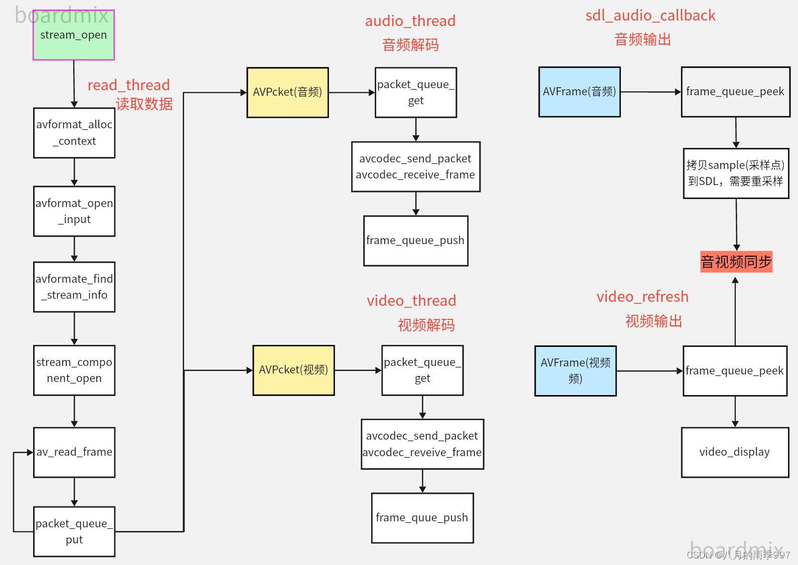
FFmpeg: 简易ijkplayer播放器实现--06封装打开和关闭stream
文章目录 流程图stream openstream close 流程图 stream open 初始化SDL以允许⾳频输出;初始化帧Frame队列初始化包Packet队列初始化时钟Clock初始化音量创建解复用读取线程read_thread创建视频刷新线程video_refresh_thread int FFPlayer::stream_open(const cha…...
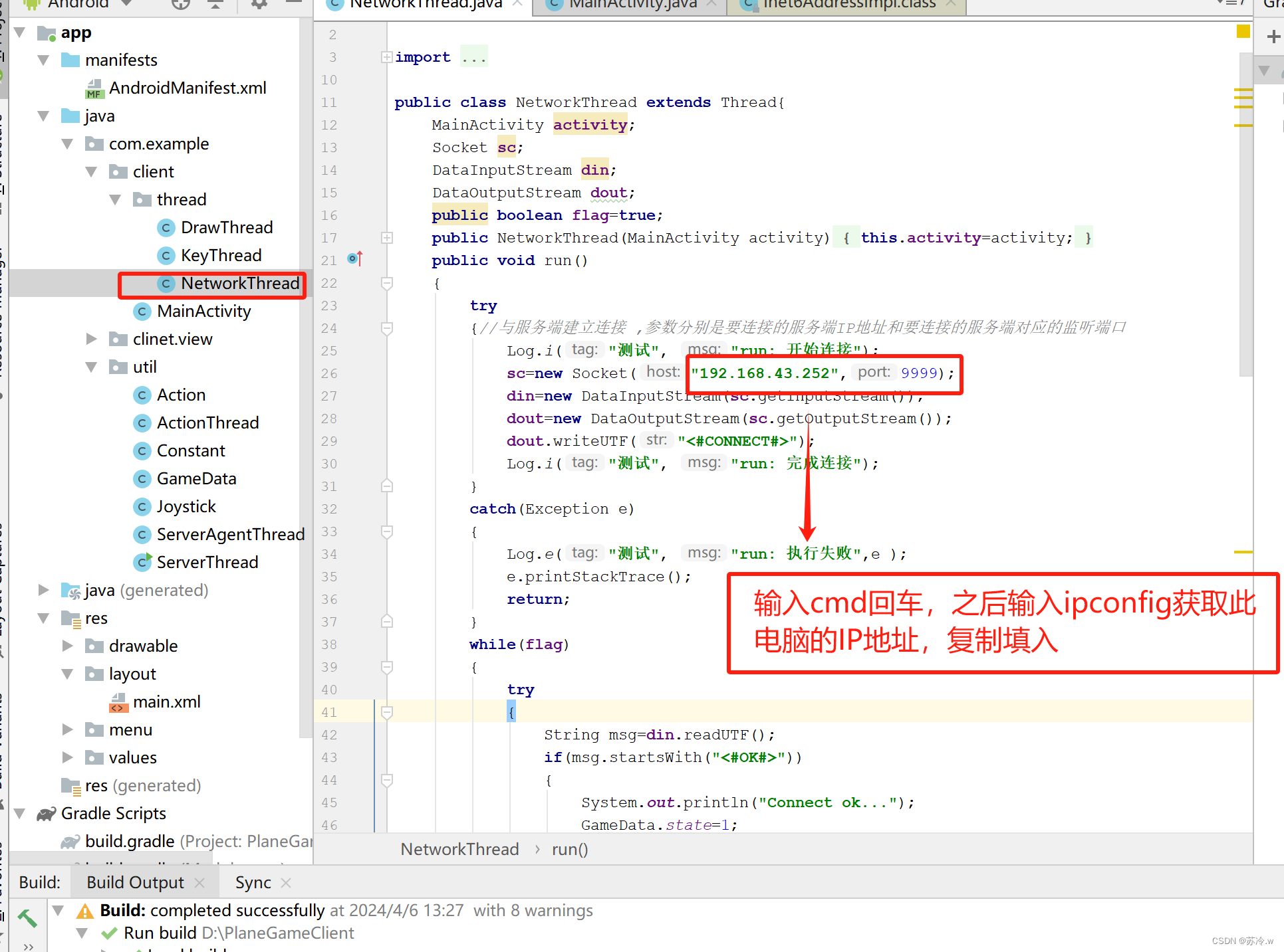
使用Android完成案例教学
目录 题目:完成在Android平台下2个玩家分别利用2个手机连接在同一局域网下通过滑动摇杆分别使红飞机和黄飞机移动的开发。(全代码解析) 题目:完成在Android平台下2个玩家分别利用2个手机连接在同一局域网下通过滑动摇杆分别使红飞…...
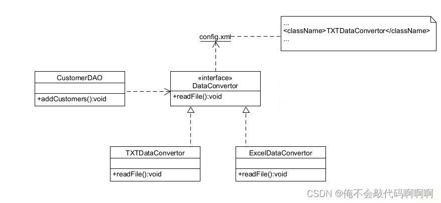
面向对象设计原则实验“依赖倒置原则”
高层模块不应该依赖于低层模块。二者都应该依赖于抽象。抽象不应该依赖于细节。细节应该依赖于抽象。 (开闭原则、里氏代换原则和依赖倒转原则的三个实例很相似,原因是它之间的关系很紧密,在实现很多重构时通常需要同时使用这三个原则。开闭…...
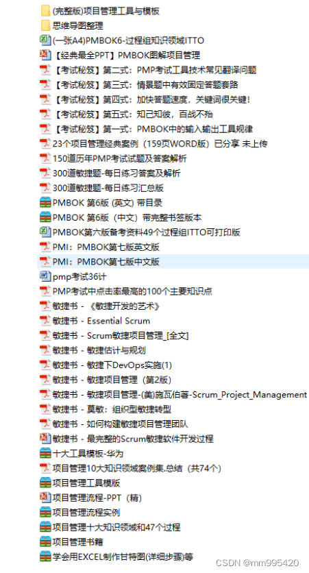
PMP考试到底难在哪里?
虽然PMP考试整体的并没有那么难,通过率也比较高,但PMP考试设计地非常巧妙,所以在面对考试时也不能掉以轻心。 01涉及面广 目前PMP考试内容大部分来源于教材《PMBOK指南》和《敏捷实践指南》。 作为考试出题的知识基础《PMBOK指南》&#x…...

Linux执行命令监控详细实现原理和使用教程,以及相关工具的使用
Linux执行命令监控详细实现原理和使用教程,以及相关工具的使用。 0x00 背景介绍 Linux上的HIDS需要实时对执行的命令进行监控,分析异常或入侵行为,有助于安全事件的发现和预防。为了获取执行命令,大致有如下方法: 遍…...
算法设计与分析实验报告c++实现(生命游戏、带锁的门、三壶谜题、串匹配问题、交替放置的碟子)
一、实验目的 1.加深学生对分治法算法设计方法的基本思想、基本步骤、基本方法的理解与掌握; 2.提高学生利用课堂所学知识解决实际问题的能力; 3.提高学生综合应用所学知识解决实际问题的能力。 二、实验任务 1、 编…...
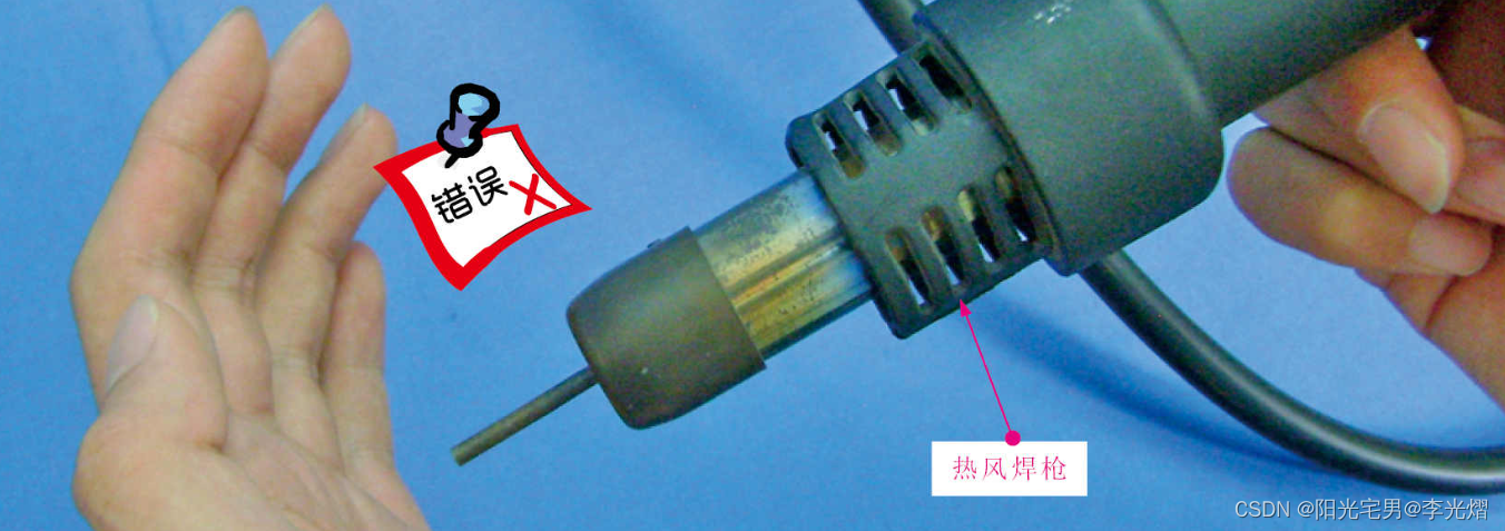
【电子通识】热风枪的结构与使用方法
热风枪的结构 热风枪是专门用来拆焊、焊接贴片元器件和贴片集成电路的焊接工具,它主要由主机和热风焊枪两大部分构成。 热风枪主要有电源开关、风速设置、温度设置、热风连接等部件组成。根据不同品牌和价位的热风枪,有一些功能齐全的也集成了烙铁功能。…...

mysql知识点
MySQL 中有哪几种锁 表级锁:开销小,加锁快;不会出现死锁;锁定粒度大,发生锁冲突的概率最高,并发度最低。行级锁:开销大,加锁慢;会出现死锁;锁定粒度最小&…...

css Animation 动画-右进左出
transform: rotate(旋转) | scale(缩放) | skew(倾斜) | translate(移动) ;<style> .jinggao {width: 60vw;display: inline-block;text-align: center;overflow: hidden;box-…...
)
第十三届蓝桥杯省赛大学B组填空题(c++)
A.扫雷 暴力模拟AC: #include<iostream> using namespace std; const int N105; int n,m,map[N][N],ans[N][N]; int dx[8]{-1,-1,0,1,1,1,0,-1}; int dy[8]{0,1,1,1,0,-1,-1,-1}; int count(int x,int y){int cnt0;for(int i0;i<8;i){int xxxdx[i];int yyydy[i];if(…...
深耕金融知识领域,助力消费者提升金融素养)
天星金融(原小米金融)深耕金融知识领域,助力消费者提升金融素养
近年来,依托生活和消费品质不断提升的时代契机,信用卡持卡人的数量以及信用卡消费的频率不断增加,信用卡还款问题也日益凸显。部分不法分子打着“智能还款”、“精养提额”的口号“踏浪”入场,实则行诱导、诈骗之实。天星金融&…...
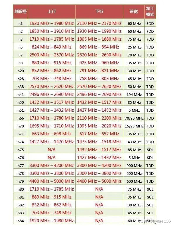
中国手机频段介绍
中国目前有三大运营商,分别是中国移动、中国联通、中国电信,还有一个潜在的运营商中国广电,各家使用的2/3/4G的制式略有不同 中国移动的GSM包括900M和1800M两个频段。 中国移动的4G的TD-LTE包括B34、B38、B39、B40、B41几个频段,…...

企业如何使用SNP Glue将SAP与Snowflake集成?
SNP Glue是SNP的集成技术,适用于任何云平台。它最初是围绕SAP和Hadoop构建的,现在已经发展为一个集成平台,虽然它仍然非常专注SAP,但可以将几乎任何数据源与任何数据目标集成。 我们客户非常感兴趣的数据目标之一是Snowflake。Sno…...
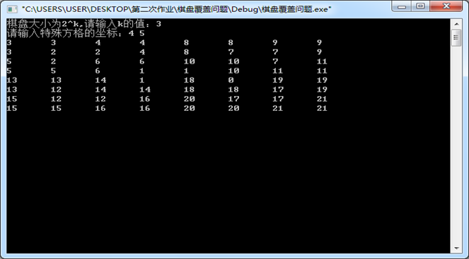
算法设计与分析实验报告c++实现(最近点对问题、循环赛日程安排问题、排序问题、棋盘覆盖问题)
一、实验目的 1.加深学生对分治法算法设计方法的基本思想、基本步骤、基本方法的理解与掌握; 2.提高学生利用课堂所学知识解决实际问题的能力; 3.提高学生综合应用所学知识解决实际问题的能力。 二、实验任务 1、最…...
Vue - 你知道Vue中computed和watch的区别吗
难度级别:中高级及以上 提问概率:70% 二者都是用来监听数据变化的,而且在日常工作中大部分时候都只是局限于简单实用,所以到了面试中很难全面说出二者的区别。接下来我们看一下,二者究竟有哪些区别呢? 先说computed,它的主要用途是监听…...
POJ2976 Dropping tests——P4377 [USACO18OPEN] Talent Show G 【分数规划二分法+贪心/背包】
POJ2976 Dropping tests 【分数规划二分法+贪心】 有 n 个物品,每个物品有两个权值 a 和b。你可以放弃 k 个物品,选 n-k 个物品,使得最大。 输入多个样例,第一行输入n 和 k,第二行输入n 个 ai ,第三行输入 n 个 bi,输入 0 0 结束。 输出答案乘100 后四舍五入到整数…...
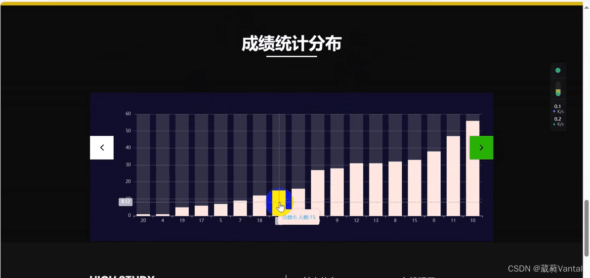
【生产实习-毕设】pyspark学生成绩分析与预测(上)
注意:数据由实习单位老师提供(需要自行搜索下载),页面美化为下载模板。 项目介绍:前端页面输入影响成绩的属性,预测出成绩,并作可视化展示——属性对成绩的影响。使用python pyspark 进行数据预…...

【华为笔试题汇总】2024-04-10-华为春招笔试题(第二套)-三语言题解(CPP/Python/Java)
🍭 大家好这里是KK爱Coding ,一枚热爱算法的程序员 ✨ 本系列打算持续跟新华为近期的春秋招笔试题汇总~ 💻 ACM银牌🥈| 多次AK大厂笔试 | 编程一对一辅导 👏 感谢大家的订阅➕ 和 喜欢…...
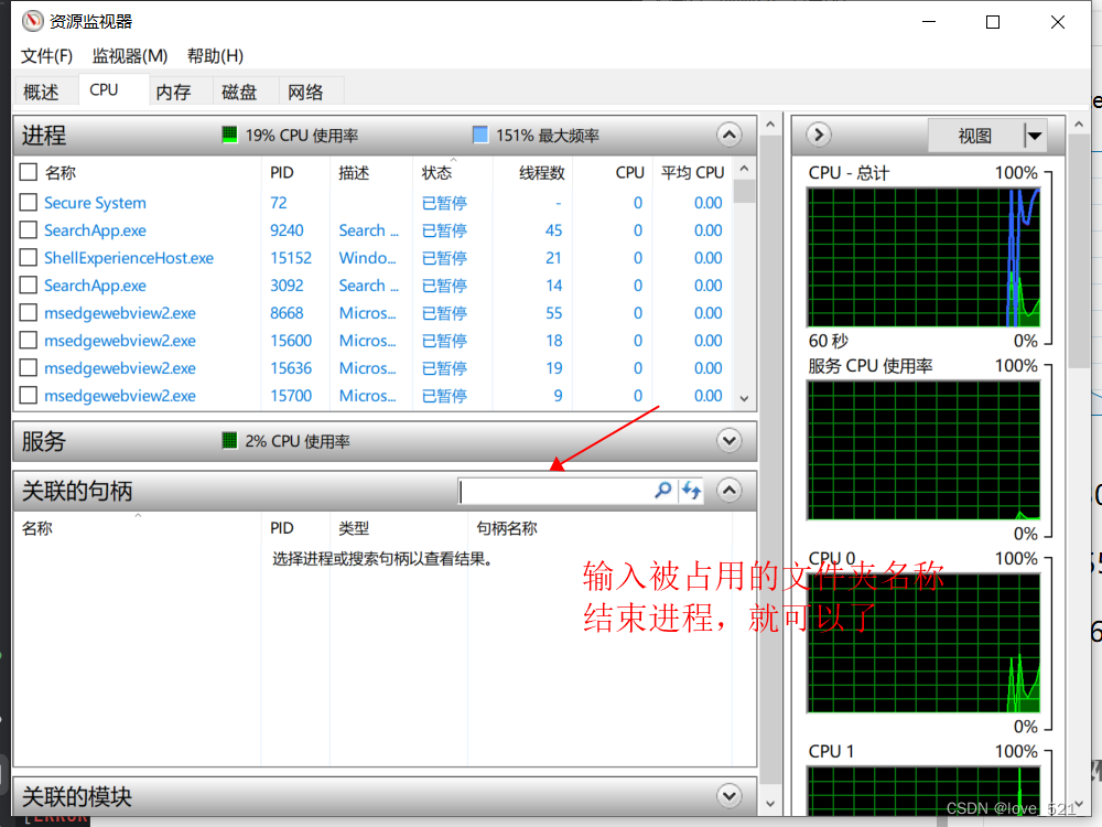
Windows 文件夹被占用无法删除
按下键盘上的“Ctrl Alt Delete”键打开任务管理器...

浅谈 React Hooks
React Hooks 是 React 16.8 引入的一组 API,用于在函数组件中使用 state 和其他 React 特性(例如生命周期方法、context 等)。Hooks 通过简洁的函数接口,解决了状态与 UI 的高度解耦,通过函数式编程范式实现更灵活 Rea…...

【网络】每天掌握一个Linux命令 - iftop
在Linux系统中,iftop是网络管理的得力助手,能实时监控网络流量、连接情况等,帮助排查网络异常。接下来从多方面详细介绍它。 目录 【网络】每天掌握一个Linux命令 - iftop工具概述安装方式核心功能基础用法进阶操作实战案例面试题场景生产场景…...
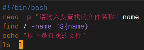
shell脚本--常见案例
1、自动备份文件或目录 2、批量重命名文件 3、查找并删除指定名称的文件: 4、批量删除文件 5、查找并替换文件内容 6、批量创建文件 7、创建文件夹并移动文件 8、在文件夹中查找文件...

全球首个30米分辨率湿地数据集(2000—2022)
数据简介 今天我们分享的数据是全球30米分辨率湿地数据集,包含8种湿地亚类,该数据以0.5X0.5的瓦片存储,我们整理了所有属于中国的瓦片名称与其对应省份,方便大家研究使用。 该数据集作为全球首个30米分辨率、覆盖2000–2022年时间…...
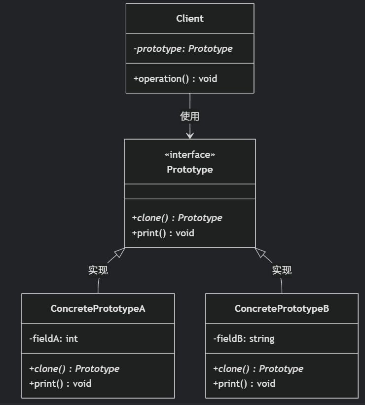
(二)原型模式
原型的功能是将一个已经存在的对象作为源目标,其余对象都是通过这个源目标创建。发挥复制的作用就是原型模式的核心思想。 一、源型模式的定义 原型模式是指第二次创建对象可以通过复制已经存在的原型对象来实现,忽略对象创建过程中的其它细节。 📌 核心特点: 避免重复初…...

镜像里切换为普通用户
如果你登录远程虚拟机默认就是 root 用户,但你不希望用 root 权限运行 ns-3(这是对的,ns3 工具会拒绝 root),你可以按以下方法创建一个 非 root 用户账号 并切换到它运行 ns-3。 一次性解决方案:创建非 roo…...

leetcodeSQL解题:3564. 季节性销售分析
leetcodeSQL解题:3564. 季节性销售分析 题目: 表:sales ---------------------- | Column Name | Type | ---------------------- | sale_id | int | | product_id | int | | sale_date | date | | quantity | int | | price | decimal | -…...

今日科技热点速览
🔥 今日科技热点速览 🎮 任天堂Switch 2 正式发售 任天堂新一代游戏主机 Switch 2 今日正式上线发售,主打更强图形性能与沉浸式体验,支持多模态交互,受到全球玩家热捧 。 🤖 人工智能持续突破 DeepSeek-R1&…...
可以参考以下方法:)
根据万维钢·精英日课6的内容,使用AI(2025)可以参考以下方法:
根据万维钢精英日课6的内容,使用AI(2025)可以参考以下方法: 四个洞见 模型已经比人聪明:以ChatGPT o3为代表的AI非常强大,能运用高级理论解释道理、引用最新学术论文,生成对顶尖科学家都有用的…...

【C++从零实现Json-Rpc框架】第六弹 —— 服务端模块划分
一、项目背景回顾 前五弹完成了Json-Rpc协议解析、请求处理、客户端调用等基础模块搭建。 本弹重点聚焦于服务端的模块划分与架构设计,提升代码结构的可维护性与扩展性。 二、服务端模块设计目标 高内聚低耦合:各模块职责清晰,便于独立开发…...