【数据挖掘】实验8:分类与预测建模
实验8:分类与预测建模
一:实验目的与要求
1:学习和掌握回归分析、决策树、人工神经网络、KNN算法、朴素贝叶斯分类等机器学习算法在R语言中的应用。
2:了解其他分类与预测算法函数。
3:学习和掌握分类与预测算法的评价。
二:实验内容
【回归分析】
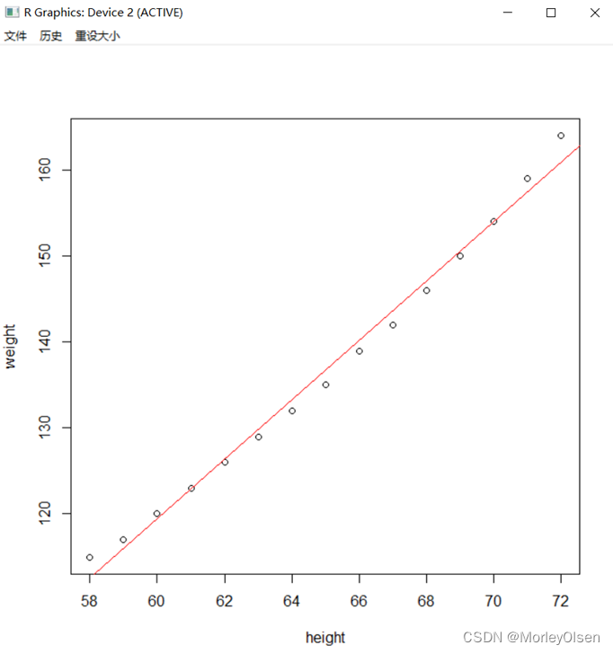
Eg.1:
| attach(women) fit<-lm(weight ~ height) plot(height,weight) abline(fit,col="red") detach(women) |
【线性回归模型】
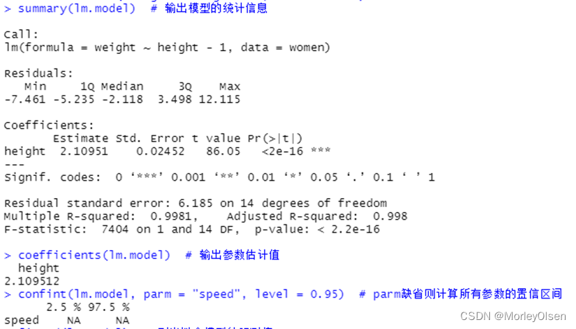
Eg.1:利用数据集women建立简单线性回归模型
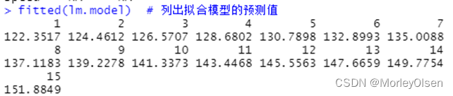
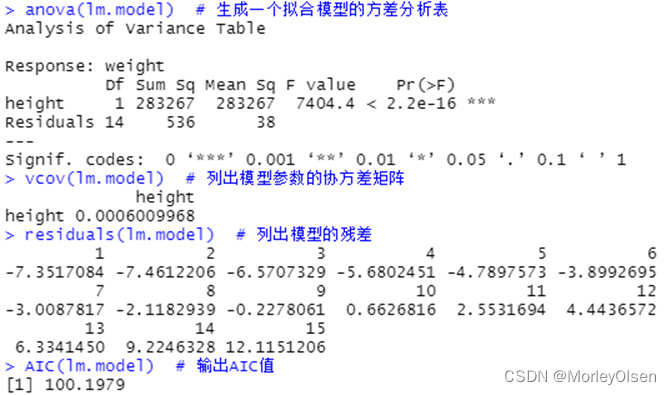
| data(women) lm.model <- lm( weight ~ height - 1, data = women) # 建立线性回归模型 summary(lm.model) # 输出模型的统计信息 coefficients(lm.model) # 输出参数估计值 confint(lm.model, parm = "speed", level = 0.95) # parm缺省则计算所有参数的置信区间 fitted(lm.model) # 列出拟合模型的预测值 anova(lm.model) # 生成一个拟合模型的方差分析表 vcov(lm.model) # 列出模型参数的协方差矩阵 residuals(lm.model) # 列出模型的残差 AIC(lm.model) # 输出AIC值 par(mfrow = c(2, 2)) plot(lm.model) # 生成评价拟合模型的诊断图 |

【逻辑回归模型】
Eg.1:结婚时间、教育、宗教等其它变量对出轨次数的影响
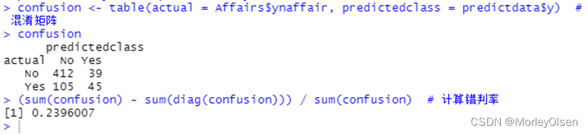
| install.packages("AER") library(AER) data(Affairs, package = "AER") # 由于变量affairs为正整数,为了进行Logistic回归先要将其转化为二元变量。 Affairs$ynaffair[Affairs$affairs > 0] <- 1 Affairs$ynaffair[Affairs$affairs == 0] <- 0 Affairs$ynaffair <- factor(Affairs$ynaffair, levels = c(0, 1), labels = c("No", "Yes")) # 建立Logistic回归模型 model.L <- glm(ynaffair ~ age + yearsmarried + religiousness + rating, data = Affairs, family = binomial (link = logit)) summary(model.L) # 展示拟合模型的详细结果 predictdata <- data.frame(Affairs[, c("age", "yearsmarried", "religiousness", "rating")]) # 由于拟合结果是给每个观测值一个概率值,下面以0.4作为分类界限 predictdata$y <- (predict(model.L, predictdata, type = "response") > 0.4) predictdata$y[which(predictdata$y == FALSE)] = "No" # 把预测结果转换成原先的值(Yes或No) predictdata$y[which(predictdata$y == TRUE)] = "Yes" confusion <- table(actual = Affairs$ynaffair, predictedclass = predictdata$y) # 混淆矩阵 confusion (sum(confusion) - sum(diag(confusion))) / sum(confusion) # 计算错判率 |


【Bonferroni离群点检验】
Eg.1:对美国妇女的平均身高和体重数据进行Bonferroni离群点检验
| install.packages("car") library(car) fit <- lm(weight ~ height, data = women) # 建立线性模型 outlierTest(fit) # Bonferroni离群点检验 women[10, ] <- c(70, 200) # 将第10个观测的数据该成height = 70,weight = 200 fit <- lm(weight ~ height, data = women) outlierTest(fit) # Bonferroni离群点检验 |

【检验误差项的自相关性】
Eg.1:对模型lm.model的误差做自相关性检验
| durbinWatsonTest(lm.model) |

【自变量选择】
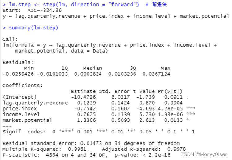
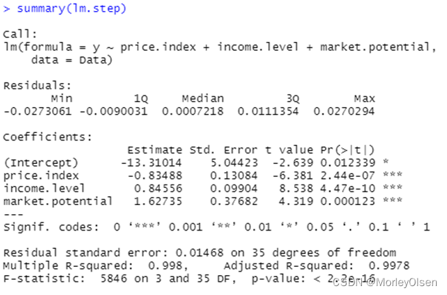
Eg.1:使用数据集freeny建立逻辑回归模型,并进行自变量选择
| Data <- freeny lm <- lm(y ~ ., data = Data) # logistic回归模型 summary(lm) lm.step <- step(lm, direction = "both") # 一切子集回归 summary(lm.step) lm.step <- step(lm, direction = "forward") # 前进法 summary(lm.step) lm.step <- step(lm, direction = "backward") # 后退法 summary(lm.step) |


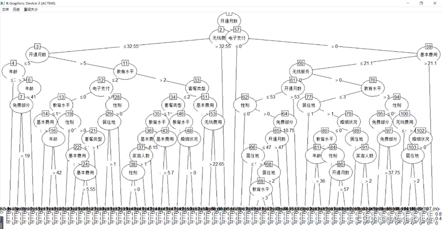
【C4.5决策树】
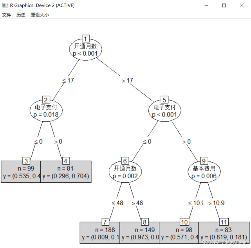
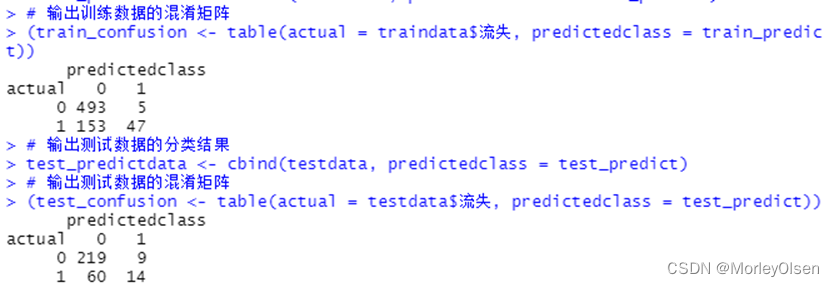
Eg.1:C4.5决策树预测客户是否流失
| Data <- read.csv("Telephone.csv",fileEncoding = "GB2312") # 读入数据 Data[, "流失"] <- as.factor(Data[, "流失"]) # 将目标变量转换成因子型 set.seed(1234) # 设置随机种子 # 数据集随机抽70%定义为训练数据集,30%为测试数据集 ind <- sample(2, nrow(Data), replace = TRUE, prob = c(0.7, 0.3)) traindata <- Data[ind == 1, ] testdata <- Data[ind == 2, ] # 建立决策树模型预测客户是否流失 install.packages("matrixStats") install.packages("party") library(party) # 加载决策树的包 ctree.model <- ctree(流失 ~ ., data = traindata) # 建立C4.5决策树模型 plot(ctree.model, type = "simple") # 输出决策树图 # 预测结果 train_predict <- predict(ctree.model) # 训练数据集 test_predict <- predict(ctree.model, newdata = testdata) # 测试数据集 # 输出训练数据的分类结果 # 输出训练数据的分类结果 train_predictdata <- cbind(traindata, predictedclass = train_predict) #输出训练数据的混淆矩阵 (train_confusion <- table(actual = traindata$流失, predictedclass = train_predict) ) # 输出测试数据的分类结果 test_predictdata <- cbind(testdata, predictedclass = test_predict) # 输出测试数据的混淆矩阵 (test_confusion <- table(actual = testdata$流失, predictedclass = test_predict)) |

【CART决策树】
Eg.1:CART决策树预测客户是否流失
| Data <- read.csv("telephone.csv",fileEncoding = "GB2312") # 读入数据 Data[, "流失"] <- as.factor(Data[, "流失"]) # 将目标变量转换成因子型 set.seed(1234) # 设置随机种子 # 数据集随机抽70%定义为训练数据集,30%为测试数据集 ind <- sample(2, nrow(Data), replace = TRUE, prob = c(0.7, 0.3)) traindata <- Data[ind == 1, ] testdata <- Data[ind == 2, ] # 建立决策树模型预测客户是否流失 install.packages("tree") library(tree) # 加载决策树的包 tree.model <- tree(流失 ~ ., data = traindata) # 建立CART决策树模型 plot(tree.model, type = "uniform") # 输出决策树图 text(tree.model) # 预测结果 train_predict <- predict(tree.model, type = "class") # 训练数据集 test_predict <- predict(tree.model, newdata = testdata, type = "class") # 测试数据集 # 输出训练数据的分类结果 train_predictdata <- cbind(traindata, predictedclass = train_predict) # 输出训练数据的混淆矩阵 (train_confusion <- table(actual = traindata$流失, predictedclass = train_predict)) # 输出测试数据的分类结果 test_predictdata <- cbind(testdata, predictedclass = test_predict) # 输出测试数据的混淆矩阵 (test_confusion <- table(actual = testdata$流失, predictedclass = test_predict)) |

【C5.0决策树】
Eg.1:C5.0决策树预测客户是否流失
| Data <- read.csv("telephone.csv",fileEncoding = "GB2312") # 读入数据 Data[, "流失"] <- as.factor(Data[, "流失"]) # 将目标变量转换成因子型 set.seed(1234) # 设置随机种子 # 数据集随机抽70%定义为训练数据集,30%为测试数据集 ind <- sample(2, nrow(Data), replace = TRUE, prob = c(0.7, 0.3)) traindata <- Data[ind == 1, ] testdata <- Data[ind == 2, ] # 建立决策树模型预测客户是否流失 install.packages("C50") library(C50) # 加载决策树的包 c50.model <- C5.0(流失 ~ ., data = traindata) # 建立C5.0决策树模型 plot(c50.model) # 输出决策树图 # 预测结果 train_predict <- predict(c50.model, newdata = traindata, type = "class") # 训练数据集 test_predict <- predict(c50.model, newdata = testdata, type = "class") # 测试数据集 # 输出训练数据的分类结果 train_predictdata <- cbind(traindata, predictedclass = train_predict) # 输出训练数据的混淆矩阵 (train_confusion <- table(actual = traindata$流失, predictedclass = train_predict)) # 输出测试数据的分类结果 test_predictdata <- cbind(testdata, predictedclass = test_predict) # 输出测试数据的混淆矩阵 (test_confusion <- table(actual = testdata$流失, predictedclass = test_predict)) |
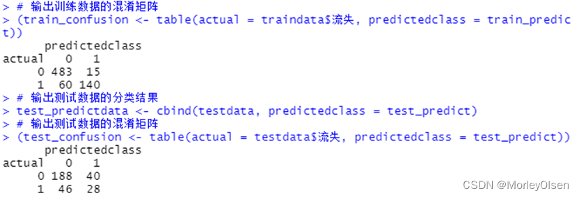
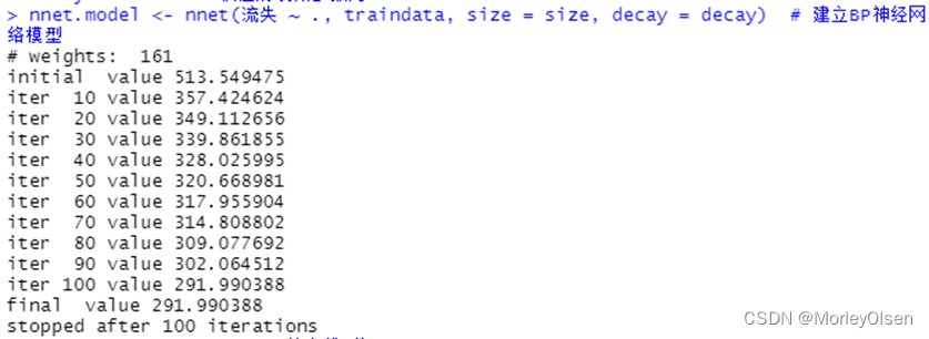
【BP神经网络】
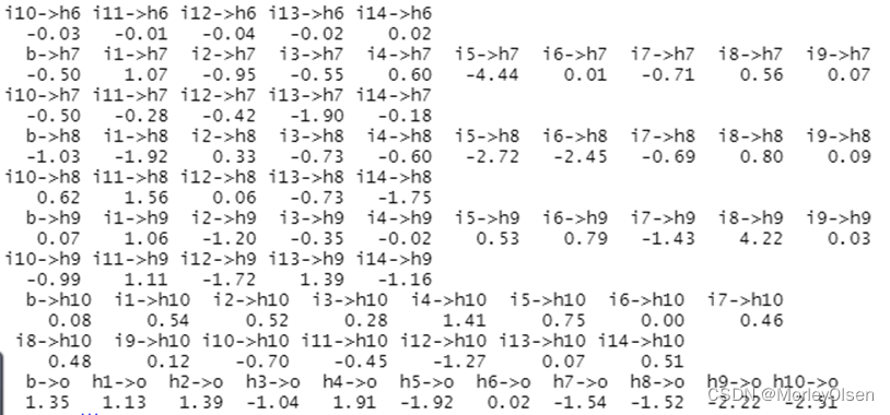
Eg.1:BP神经网络算法预测客户是否流失
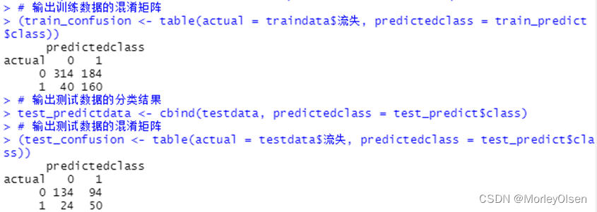
| Data[, "流失"] <- as.factor(Data[, "流失"]) # 将目标变量转换成因子型 set.seed(1234) # 设置随机种子 # 数据集随机抽70%定义为训练数据集,30%为测试数据集 ind <- sample(2, nrow(Data), replace = TRUE, prob = c(0.7, 0.3)) traindata <- Data[ind == 1, ] testdata <- Data[ind == 2, ] # BP神经网络建模 library(nnet) #加载nnet包 # 设置参数 size <- 10 # 隐层节点数为10 decay <- 0.05 # 权值的衰减参数为0.05 nnet.model <- nnet(流失 ~ ., traindata, size = size, decay = decay) # 建立BP神经网络模型 summary(nnet.model) # 输出模型概要 # 预测结果 train_predict <- predict(nnet.model, newdata = traindata, type = "class") # 训练数据集 test_predict <- predict(nnet.model, newdata = testdata, type = "class") # 测试数据集 # 输出训练数据的分类结果 train_predictdata <- cbind(traindata, predictedclass = train_predict) # 输出训练数据的混淆矩阵 (train_confusion <- table(actual = traindata$流失, predictedclass = train_predict)) # 输出测试数据的分类结果 test_predictdata <- cbind(testdata, predictedclass = test_predict) # 输出测试数据的混淆矩阵 (test_confusion <- table(actual = testdata$流失, predictedclass = test_predict)) |


【KNN算法】
Eg.1:KNN算法预测客户是否流失
| Data[, "流失"] <- as.factor(Data[, "流失"]) # 将目标变量转换成因子型 set.seed(1234) # 设置随机种子 # 数据集随机抽70%定义为训练数据集,30%为测试数据集 ind <- sample(2, nrow(Data), replace = TRUE, prob = c(0.7, 0.3)) traindata <- Data[ind == 1, ] testdata <- Data[ind == 2, ] # 使用kknn函数建立knn分类模型 install.packages("kknn") library(kknn) # 加载kknn包 # knn分类模型 kknn.model <- kknn(流失 ~ ., train = traindata, test = traindata, k = 5) # 训练数据 kknn.model2 <- kknn(流失 ~ ., train = traindata, test = testdata, k = 5) # 测试数据 summary(kknn.model) # 输出模型概要 # 预测结果 train_predict <- predict(kknn.model) # 训练数据 test_predict <- predict(kknn.model2) # 测试数据 # 输出训练数据的混淆矩阵 (train_confusion <- table(actual = traindata$流失, predictedclass = train_predict)) # 输出测试数据的混淆矩阵 (test_confusion <- table(actual = testdata$流失, predictedclass = test_predict)) # 使用knn函数建立knn分类模型 library(class) # 加载class包 # 建立knn分类模型 knn.model <- knn(traindata, testdata, cl = traindata[, "流失"]) # 输出测试数据的混淆矩阵 (test_confusion = table(actual = testdata$流失, predictedclass = knn.model)) # 使用train函数建立knn分类模型 install.packages("caret") library(caret) # 加载caret包 # 建立knn分类模型 train.model <- train(traindata, traindata[, "流失"], method = "knn") # 预测结果 train_predict <- predict(train.model, newdata = traindata) #训练数据集 test_predict <- predict(train.model, newdata = testdata) #测试数据集 # 输出训练数据的混淆矩阵 (train_confusion <- table(actual = traindata$流失, predictedclass = train_predict)) # 输出测试数据的混淆矩阵 (test_confusion <- table(actual = testdata$流失, predictedclass = test_predict)) |
运行结果:
| 模型概要输出 |
| Call: kknn(formula = 流失 ~ ., train = traindata, test = traindata, k = 5) Response: "nominal" fit prob.0 prob.1 1 1 0.33609798 0.66390202 2 1 0.25597771 0.74402229 3 0 0.97569952 0.02430048 4 0 0.51243637 0.48756363 5 0 1.00000000 0.00000000 6 1 0.17633839 0.82366161 7 0 0.59198438 0.40801562 8 0 1.00000000 0.00000000 9 0 1.00000000 0.00000000 10 1 0.36039846 0.63960154 11 0 0.74402229 0.25597771 12 0 0.84796209 0.15203791 13 0 0.89557925 0.10442075 14 0 1.00000000 0.00000000 15 0 1.00000000 0.00000000 16 0 0.74402229 0.25597771 17 1 0.02430048 0.97569952 18 1 0.15203791 0.84796209 19 0 1.00000000 0.00000000 20 0 0.97569952 0.02430048 21 0 0.97569952 0.02430048 22 0 1.00000000 0.00000000 23 0 0.76784183 0.23215817 24 0 0.74354135 0.25645865 25 0 0.74402229 0.25597771 26 0 1.00000000 0.00000000 27 0 1.00000000 0.00000000 28 0 0.51186411 0.48813589 29 0 1.00000000 0.00000000 30 0 0.97569952 0.02430048 31 0 1.00000000 0.00000000 32 0 0.56768390 0.43231610 33 0 0.84796209 0.15203791 34 0 0.66390202 0.33609798 35 1 0.00000000 1.00000000 36 0 1.00000000 0.00000000 37 0 1.00000000 0.00000000 38 0 0.84796209 0.15203791 39 1 0.25597771 0.74402229 40 1 0.48813589 0.51186411 41 1 0.36039846 0.63960154 42 0 0.97569952 0.02430048 43 0 0.89557925 0.10442075 44 0 1.00000000 0.00000000 45 0 0.51243637 0.48756363 46 0 0.66390202 0.33609798 47 0 0.74402229 0.25597771 48 0 1.00000000 0.00000000 49 0 1.00000000 0.00000000 50 0 1.00000000 0.00000000 51 1 0.36039846 0.63960154 52 0 0.91987973 0.08012027 53 0 1.00000000 0.00000000 54 0 0.91987973 0.08012027 55 1 0.25597771 0.74402229 56 0 0.89557925 0.10442075 57 0 0.91987973 0.08012027 58 0 1.00000000 0.00000000 59 0 0.56768390 0.43231610 60 1 0.48813589 0.51186411 61 0 1.00000000 0.00000000 62 0 1.00000000 0.00000000 63 1 0.48756363 0.51243637 64 0 0.51243637 0.48756363 65 0 0.51243637 0.48756363 66 0 0.84796209 0.15203791 67 0 0.84796209 0.15203791 68 0 0.76784183 0.23215817 69 1 0.02430048 0.97569952 70 1 0.00000000 1.00000000 71 0 0.84796209 0.15203791 72 0 0.76784183 0.23215817 73 0 0.76784183 0.23215817 74 1 0.15203791 0.84796209 75 1 0.02430048 0.97569952 76 0 1.00000000 0.00000000 77 0 0.51243637 0.48756363 78 1 0.36039846 0.63960154 79 0 0.71972181 0.28027819 80 0 0.82366161 0.17633839 81 1 0.36039846 0.63960154 82 1 0.23215817 0.76784183 83 0 0.76784183 0.23215817 84 1 0.00000000 1.00000000 85 0 1.00000000 0.00000000 86 0 0.66390202 0.33609798 87 0 1.00000000 0.00000000 88 0 0.91987973 0.08012027 89 1 0.23215817 0.76784183 90 0 1.00000000 0.00000000 91 0 0.91987973 0.08012027 92 0 1.00000000 0.00000000 93 0 1.00000000 0.00000000 94 1 0.10442075 0.89557925 95 0 0.91987973 0.08012027 96 0 0.74354135 0.25645865 97 1 0.25645865 0.74354135 98 1 0.33609798 0.66390202 99 0 0.91987973 0.08012027 100 1 0.25645865 0.74354135 101 0 1.00000000 0.00000000 102 1 0.28027819 0.71972181 103 0 0.66390202 0.33609798 104 0 0.51186411 0.48813589 105 0 0.56768390 0.43231610 106 0 0.84796209 0.15203791 107 0 0.76784183 0.23215817 108 0 1.00000000 0.00000000 109 0 0.76784183 0.23215817 110 0 0.91987973 0.08012027 111 1 0.43231610 0.56768390 112 0 1.00000000 0.00000000 113 0 0.97569952 0.02430048 114 0 1.00000000 0.00000000 115 0 0.76784183 0.23215817 116 0 0.63960154 0.36039846 117 0 0.97569952 0.02430048 118 1 0.15203791 0.84796209 119 0 0.74402229 0.25597771 120 0 1.00000000 0.00000000 121 0 1.00000000 0.00000000 122 0 0.91987973 0.08012027 123 0 1.00000000 0.00000000 124 0 0.74354135 0.25645865 125 0 1.00000000 0.00000000 126 1 0.43231610 0.56768390 127 0 0.71972181 0.28027819 128 1 0.08012027 0.91987973 129 0 0.91987973 0.08012027 130 1 0.10442075 0.89557925 131 0 1.00000000 0.00000000 132 0 0.91987973 0.08012027 133 0 0.51243637 0.48756363 134 0 0.66390202 0.33609798 135 1 0.02430048 0.97569952 136 0 1.00000000 0.00000000 137 0 0.74354135 0.25645865 138 0 0.97569952 0.02430048 139 0 1.00000000 0.00000000 140 0 1.00000000 0.00000000 141 1 0.25597771 0.74402229 142 0 1.00000000 0.00000000 143 0 1.00000000 0.00000000 144 1 0.36039846 0.63960154 145 0 1.00000000 0.00000000 146 0 0.74402229 0.25597771 147 0 0.84796209 0.15203791 148 0 0.91987973 0.08012027 149 0 0.51243637 0.48756363 150 0 1.00000000 0.00000000 151 1 0.28027819 0.71972181 152 0 1.00000000 0.00000000 153 0 0.59198438 0.40801562 154 0 0.51243637 0.48756363 155 1 0.33609798 0.66390202 156 0 0.97569952 0.02430048 157 0 1.00000000 0.00000000 158 0 1.00000000 0.00000000 159 0 0.59198438 0.40801562 160 1 0.48756363 0.51243637 161 0 1.00000000 0.00000000 162 0 0.97569952 0.02430048 163 1 0.25645865 0.74354135 164 1 0.33609798 0.66390202 165 0 0.51186411 0.48813589 166 1 0.43231610 0.56768390 167 0 1.00000000 0.00000000 168 0 1.00000000 0.00000000 169 0 1.00000000 0.00000000 170 0 1.00000000 0.00000000 171 0 1.00000000 0.00000000 172 0 0.76784183 0.23215817 173 0 0.56768390 0.43231610 174 0 0.76784183 0.23215817 175 0 0.84796209 0.15203791 176 0 1.00000000 0.00000000 177 0 0.51243637 0.48756363 178 0 0.51243637 0.48756363 179 0 0.63960154 0.36039846 180 0 0.74402229 0.25597771 181 0 1.00000000 0.00000000 182 1 0.15203791 0.84796209 183 0 0.66390202 0.33609798 184 1 0.02430048 0.97569952 185 0 0.97569952 0.02430048 186 1 0.23215817 0.76784183 187 0 0.97569952 0.02430048 188 0 0.51186411 0.48813589 189 1 0.25597771 0.74402229 190 0 1.00000000 0.00000000 191 0 1.00000000 0.00000000 192 0 1.00000000 0.00000000 193 0 1.00000000 0.00000000 194 0 1.00000000 0.00000000 195 0 0.91987973 0.08012027 196 0 1.00000000 0.00000000 197 0 0.91987973 0.08012027 198 0 0.74402229 0.25597771 199 0 1.00000000 0.00000000 200 0 1.00000000 0.00000000 201 0 1.00000000 0.00000000 202 0 1.00000000 0.00000000 203 0 0.97569952 0.02430048 204 0 0.84796209 0.15203791 205 1 0.00000000 1.00000000 206 0 0.89557925 0.10442075 207 0 1.00000000 0.00000000 208 0 1.00000000 0.00000000 209 0 0.91987973 0.08012027 210 0 0.84796209 0.15203791 211 0 1.00000000 0.00000000 212 0 0.74402229 0.25597771 213 0 0.74402229 0.25597771 214 0 0.66390202 0.33609798 215 0 1.00000000 0.00000000 216 0 0.91987973 0.08012027 217 0 1.00000000 0.00000000 218 0 1.00000000 0.00000000 219 0 0.51186411 0.48813589 220 0 1.00000000 0.00000000 221 1 0.00000000 1.00000000 222 1 0.15203791 0.84796209 223 0 0.51243637 0.48756363 224 1 0.28027819 0.71972181 225 1 0.08012027 0.91987973 226 0 1.00000000 0.00000000 227 0 1.00000000 0.00000000 228 1 0.25597771 0.74402229 229 1 0.15203791 0.84796209 230 1 0.15203791 0.84796209 231 0 0.51243637 0.48756363 232 1 0.08012027 0.91987973 233 1 0.28027819 0.71972181 234 1 0.40801562 0.59198438 235 0 0.51186411 0.48813589 236 0 1.00000000 0.00000000 237 1 0.43231610 0.56768390 238 0 0.89557925 0.10442075 239 1 0.33609798 0.66390202 240 0 0.74354135 0.25645865 241 0 0.97569952 0.02430048 242 0 1.00000000 0.00000000 243 0 0.97569952 0.02430048 244 0 0.89557925 0.10442075 245 0 0.74402229 0.25597771 246 0 1.00000000 0.00000000 247 0 1.00000000 0.00000000 248 0 0.84796209 0.15203791 249 1 0.36039846 0.63960154 250 0 0.84796209 0.15203791 251 1 0.48813589 0.51186411 252 0 1.00000000 0.00000000 253 0 1.00000000 0.00000000 254 0 0.91987973 0.08012027 255 0 0.56768390 0.43231610 256 0 1.00000000 0.00000000 257 0 0.84796209 0.15203791 258 1 0.33609798 0.66390202 259 0 0.76784183 0.23215817 260 0 1.00000000 0.00000000 261 1 0.36039846 0.63960154 262 0 1.00000000 0.00000000 263 0 1.00000000 0.00000000 264 1 0.48756363 0.51243637 265 1 0.48756363 0.51243637 266 0 0.89557925 0.10442075 267 0 1.00000000 0.00000000 268 0 0.66390202 0.33609798 269 0 0.56768390 0.43231610 270 0 0.74402229 0.25597771 271 1 0.25597771 0.74402229 272 0 1.00000000 0.00000000 273 0 0.66390202 0.33609798 274 0 1.00000000 0.00000000 275 0 1.00000000 0.00000000 276 0 0.89557925 0.10442075 277 0 1.00000000 0.00000000 278 0 0.51243637 0.48756363 279 0 0.84796209 0.15203791 280 0 1.00000000 0.00000000 281 0 0.84796209 0.15203791 282 0 0.91987973 0.08012027 283 0 1.00000000 0.00000000 284 0 1.00000000 0.00000000 285 0 0.97569952 0.02430048 286 0 1.00000000 0.00000000 287 0 1.00000000 0.00000000 288 0 1.00000000 0.00000000 289 0 1.00000000 0.00000000 290 0 0.91987973 0.08012027 291 0 1.00000000 0.00000000 292 0 1.00000000 0.00000000 293 0 0.91987973 0.08012027 294 0 0.76784183 0.23215817 295 1 0.17633839 0.82366161 296 1 0.10442075 0.89557925 297 0 0.84796209 0.15203791 298 0 0.97569952 0.02430048 299 1 0.36039846 0.63960154 300 0 1.00000000 0.00000000 301 0 0.84796209 0.15203791 302 0 0.91987973 0.08012027 303 0 0.89557925 0.10442075 304 0 0.97569952 0.02430048 305 0 1.00000000 0.00000000 306 1 0.02430048 0.97569952 307 1 0.15203791 0.84796209 308 1 0.40801562 0.59198438 309 0 0.84796209 0.15203791 310 1 0.00000000 1.00000000 311 0 0.89557925 0.10442075 312 0 1.00000000 0.00000000 313 0 1.00000000 0.00000000 314 1 0.48756363 0.51243637 315 0 0.51243637 0.48756363 316 0 0.97569952 0.02430048 317 0 1.00000000 0.00000000 318 0 0.97569952 0.02430048 319 1 0.25645865 0.74354135 320 0 1.00000000 0.00000000 321 1 0.08012027 0.91987973 322 1 0.33609798 0.66390202 323 0 0.91987973 0.08012027 324 0 0.89557925 0.10442075 325 0 0.91987973 0.08012027 326 0 1.00000000 0.00000000 327 1 0.25597771 0.74402229 328 0 1.00000000 0.00000000 329 0 1.00000000 0.00000000 330 1 0.43231610 0.56768390 331 0 0.84796209 0.15203791 332 0 0.51243637 0.48756363 333 1 0.33609798 0.66390202 [ reached 'max' / getOption("max.print") -- omitted 365 rows ] |


【朴素贝叶斯分类算法】
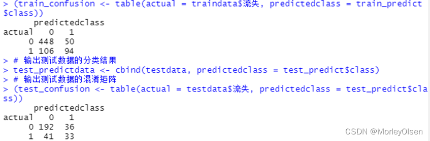
Eg.1:朴素贝叶斯算法预测客户是否流失
| Data[, "流失"] <- as.factor(Data[, "流失"]) # 将目标变量转换成因子型 set.seed(1234) # 设置随机种子 # 数据集随机抽70%定义为训练数据集,30%为测试数据集 ind <- sample(2, nrow(Data), replace = TRUE, prob = c(0.7, 0.3)) traindata <- Data[ind == 1, ] testdata <- Data[ind == 2, ] # 使用naiveBayes函数建立朴素贝叶斯分类模型 library(e1071) # 加载e1071包 naiveBayes.model <- naiveBayes(流失 ~ ., data = traindata) # 建立朴素贝叶斯分类模型 # 预测结果 train_predict <- predict(naiveBayes.model, newdata = traindata) # 训练数据集 test_predict <- predict(naiveBayes.model, newdata = testdata) # 测试数据集 # 输出训练数据的分类结果 train_predictdata <- cbind(traindata, predictedclass = train_predict) # 输出训练数据的混淆矩阵 (train_confusion <- table(actual = traindata$流失, predictedclass = train_predict)) # 输出测试数据的分类结果 test_predictdata <- cbind(testdata, predictedclass = test_predict) # 输出测试数据的混淆矩阵 (test_confusion <- table(actual = testdata$流失, predictedclass = test_predict)) # 使用NaiveBayes函数建立朴素贝叶斯分类模型 install.packages("klaR") library(klaR) # 加载klaR包 NaiveBayes.model <- NaiveBayes(流失 ~ ., data = traindata) # 建立朴素贝叶斯分类模型 # 预测结果 train_predict <- predict(NaiveBayes.model) # 训练数据集 test_predict <- predict(NaiveBayes.model, newdata = testdata) # 测试数据集 # 输出训练数据的分类结果 train_predictdata <- cbind(traindata, predictedclass = train_predict$class) # 输出训练数据的混淆矩阵 (train_confusion <- table(actual = traindata$流失, predictedclass = train_predict$class)) # 输出测试数据的分类结果 test_predictdata <- cbind(testdata, predictedclass = test_predict$class) # 输出测试数据的混淆矩阵 (test_confusion <- table(actual = testdata$流失, predictedclass = test_predict$class)) |

【lda模型】
Eg.1:建立lda模型并进行分类预测
| Data[, "流失"] <- as.factor(Data[, "流失"]) #将目标变量转换成因子型 set.seed(1234) # 设置随机种子 # 数据集随机抽70%定义为训练数据集,30%为测试数据集 ind <- sample(2, nrow(Data), replace = TRUE, prob = c(0.7, 0.3)) traindata <- Data[ind == 1, ] testdata <- Data[ind == 2, ] # 建立lda分类模型 install.packages("MASS") library(MASS) lda.model <- lda(流失 ~ ., data = traindata) # 预测结果 train_predict <- predict(lda.model, newdata = traindata) # 训练数据集 test_predict <- predict(lda.model, newdata = testdata) # 测试数据集 # 输出训练数据的分类结果 train_predictdata <- cbind(traindata, predictedclass = train_predict$class) # 输出训练数据的混淆矩阵 (train_confusion <- table(actual = traindata$流失, predictedclass = train_predict$class)) # 输出测试数据的分类结果 test_predictdata <- cbind(testdata, predictedclass = test_predict$class) # 输出测试数据的混淆矩阵 (test_confusion <- table(actual = testdata$流失, predictedclass = test_predict$class)) |
【rpart模型】
Eg.1:构建rpart模型并进行分类预测
| Data[, "流失"] <- as.factor(Data[, "流失"]) # 将目标变量转换成因子型 set.seed(1234) # 设置随机种子 # 数据集随机抽70%定义为训练数据集,30%为测试数据集 ind <- sample(2, nrow(Data), replace = TRUE, prob = c(0.7, 0.3)) traindata <- Data[ind == 1, ] testdata <- Data[ind == 2, ] # 建立rpart分类模型 library(rpart) install.packages("rpart.plot") library(rpart.plot) rpart.model <- rpart(流失 ~ ., data = traindata, method = "class", cp = 0.03) # cp为复杂的参数 # 输出决策树图 rpart.plot(rpart.model, branch = 1, branch.type = 2, type = 1, extra = 102, border.col = "blue", split.col = "red", split.cex = 1, main = "客户流失决策树") # 预测结果 train_predict <- predict(rpart.model, newdata = traindata, type = "class") # 训练数据集 test_predict <- predict(rpart.model, newdata = testdata, type = "class") # 测试数据集 # 输出训练数据的分类结果 train_predictdata <- cbind(traindata, predictedclass = train_predict) # 输出训练数据的混淆矩阵 (train_confusion <- table(actual = traindata$流失, predictedclass = train_predict)) # 输出测试数据的分类结果 test_predictdata <- cbind(testdata, predictedclass = test_predict) # 输出测试数据的混淆矩阵 (test_confusion <- table(actual = testdata$流失, predictedclass = test_predict)) |


【bagging模型】
Eg.1:构建bagging模型并进行分类预测
| Data[, "流失"] <- as.factor(Data[, "流失"]) # 将目标变量转换成因子型 set.seed(1234) # 设置随机种子 # 数据集随机抽70%定义为训练数据集,30%为测试数据集 ind <- sample(2, nrow(Data), replace = TRUE, prob = c(0.7, 0.3)) traindata <- Data[ind == 1, ] testdata <- Data[ind == 2, ] # 建立bagging分类模型 install.packages("adabag") library(adabag) bagging.model <- bagging(流失 ~ ., data = traindata) # 预测结果 train_predict <- predict(bagging.model, newdata = traindata) # 训练数据集 test_predict <- predict(bagging.model, newdata = testdata) # 测试数据集 # 输出训练数据的分类结果 train_predictdata <- cbind(traindata, predictedclass = train_predict$class) # 输出训练数据的混淆矩阵 (train_confusion <- table(actual = traindata$流失, predictedclass = train_predict$class)) # 输出测试数据的分类结果 test_predictdata <- cbind(testdata, predictedclass = test_predict$class) # 输出测试数据的混淆矩阵 (test_confusion <- table(actual = testdata$流失, predictedclass = test_predict$class)) |

【randomForest模型】
Eg.1:构建randomForest模型并进行分类预测
| Data[, "流失"] <- as.factor(Data[, "流失"]) # 将目标变量转换成因子型 set.seed(1234) # 设置随机种子 # 数据集随机抽70%定义为训练数据集,30%为测试数据集 ind <- sample(2, nrow(Data), replace = TRUE, prob = c(0.7, 0.3)) traindata <- Data[ind == 1, ] testdata <- Data[ind == 2, ] # 建立randomForest模型 install.packages("randomForest") library(randomForest) randomForest.model <- randomForest(流失 ~ ., data = traindata) # 预测结果 test_predict <- predict(randomForest.model, newdata = testdata) # 测试数据集 # 输出训练数据的混淆矩阵 (train_confusion <- randomForest.model$confusion) # 输出测试数据的混淆矩阵 (test_confusion <- table(actual = testdata$流失, predictedclass = test_predict)) |

【svm模型】
Eg.1:构建svm模型并进行分类预测
| Data[, "流失"] = as.factor(Data[, "流失"]) # 将目标变量转换成因子型 set.seed(1234) # 设置随机种子 # 数据集随机抽70%定义为训练数据集,30%为测试数据集 ind <- sample(2, nrow(Data), replace = TRUE, prob = c(0.7, 0.3)) traindata <- Data[ind == 1, ] testdata <- Data[ind == 2, ] # 建立svm模型 install.packages("e1071") library(e1071) svm.model <- svm(流失 ~ ., data = traindata) # 预测结果 train_predict <- predict(svm.model, newdata = traindata) # 训练数据集 test_predict <- predict(svm.model, newdata = testdata) # 测试数据集 # 输出训练数据的分类结果 train_predictdata <- cbind(traindata, predictedclass = train_predict) # 输出训练数据的混淆矩阵 (train_confusion <- table(actual = traindata$流失, predictedclass = train_predict)) # 输出测试数据的分类结果 test_predictdata <- cbind(testdata, predictedclass = test_predict) # 输出测试数据的混淆矩阵 (test_confusion <- table(actual = testdata$流失, predictedclass = test_predict)) |

【ROC曲线和PR曲线】
Eg.1:ROC曲线和PR曲线图代码
| install.packages("ROCR") library(ROCR) library(gplots) # 预测结果 train_predict <- predict(lda.model, newdata = traindata) # 训练数据集 test_predict <- predict(lda.model, newdata = testdata) # 测试数据集 par(mfrow = c(1, 2)) # ROC曲线 # 训练集 predi <- prediction(train_predict$posterior[, 2], traindata$流失) perfor <- performance(predi, "tpr", "fpr") plot(perfor, col = "red", type = "l", main = "ROC曲线", lty = 1) # 训练集的ROC曲线 # 测试集 predi2 <- prediction(test_predict$posterior[, 2], testdata$流失) perfor2 <- performance(predi2, "tpr", "fpr") par(new = T) plot(perfor2, col = "blue", type = "l", pch = 2, lty = 2) # 测试集的ROC曲线 abline(0, 1) legend("bottomright", legend = c("训练集", "测试集"), bty = "n", lty = c(1, 2), col = c("red", "blue")) # 图例 # PR曲线 # 训练集 perfor <- performance(predi, "prec", "rec") plot(perfor, col = "red", type = "l", main = "PR曲线", xlim = c(0, 1), ylim = c(0, 1), lty = 1) # 训练集的PR曲线 # 测试集 perfor2 <- performance(predi2, "prec", "rec") par(new = T) plot(perfor2, col = "blue", type = "l", pch = 2, xlim = c(0, 1), ylim = c(0, 1), lty = 2) # 测试集的PR曲线 abline(1, -1) legend("bottomleft", legend = c("训练集", "测试集"), bty = "n", lty = c(1, 2), col = c("red", "blue")) # 图例 |

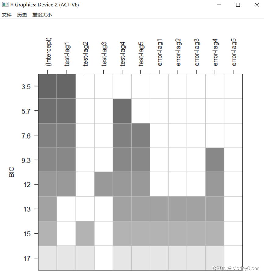
【BIC图和一阶差分】
Eg.1:
| install.packages("TSA") library(TSA) Data <- read.csv("arima_data.csv", header = T,fileEncoding = "GB2312")[, 2] sales <- ts(Data) plot.ts(sales, xlab = "时间", ylab = "销量 / 元") # 一阶差分 difsales <- diff(sales) # BIC图 res <- armasubsets(y = difsales, nar = 5, nma = 5, y.name = 'test', ar.method = 'ols') plot(res) |

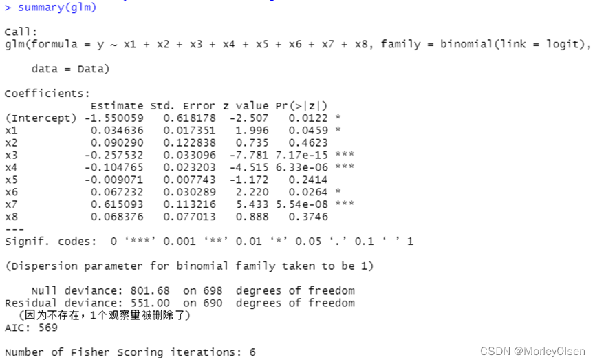
【逻辑回归】
Eg.1:
| Data <- read.csv("bankloan.csv",fileEncoding = "GB2312")[2:701, ] # 数据命名 colnames(Data) <- c("x1", "x2", "x3", "x4", "x5", "x6", "x7", "x8", "y") # logistic回归模型 glm <- glm(y ~ x1 + x2 + x3 + x4 + x5 + x6 + x7 + x8, family = binomial(link = logit), data = Data) summary(glm) # 逐步寻优法 logit.step <- step(glm, direction = "both") summary(logit.step) # 前向选择法 logit.step <- step(glm, direction = "forward") summary(logit.step) # 后向选择法 logit.step <- step(glm, direction = "backward") summary(logit.step) |


【ID3_decision_tree】
Eg.1:
| data <- read.csv("sales_data.csv",fileEncoding = "GB2312")[, 2:5] # 数据命名 colnames(data) <- c("x1", "x2", "x3", "result") # 计算一列数据的信息熵 calculateEntropy <- function(data) { t <- table(data) sum <- sum(t) t <- t[t != 0] entropy <- -sum(log2(t / sum) * (t / sum)) return(entropy) } # 计算两列数据的信息熵 calculateEntropy2 <- function(data) { var <- table(data[1]) p <- var/sum(var) varnames <- names(var) array <- c() for (name in varnames) { array <- append(array, calculateEntropy(subset(data, data[1] == name, select = 2))) } return(sum(array * p)) } buildTree <- function(data) { if (length(unique(data$result)) == 1) { cat(data$result[1]) return() } if (length(names(data)) == 1) { cat("...") return() } entropy <- calculateEntropy(data$result) labels <- names(data) label <- "" temp <- Inf subentropy <- c() for (i in 1:(length(data) - 1)) { temp2 <- calculateEntropy2(data[c(i, length(labels))]) if (temp2 < temp) { temp <- temp2 label <- labels[i] } subentropy <- append(subentropy,temp2) } cat(label) cat("[") nextLabels <- labels[labels != label] for (value in unlist(unique(data[label]))) { cat(value,":") buildTree(subset(data,data[label] == value, select = nextLabels)) cat(";") } cat("]") } # 构建分类树 buildTree(data) |

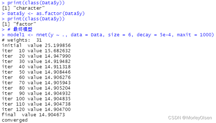
【bp_neural_network】
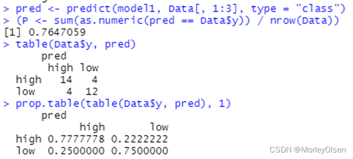
Eg.1:
| Data <- read.csv("sales_data.csv",fileEncoding = "GB2312")[, 2:5] # 数据命名 library(nnet) colnames(Data) <- c("x1", "x2", "x3", "y") print(names(Data)) print(class(Data$y)) Data$y <- as.factor(Data$y) print(class(Data$y)) # 最终模型 model1 <- nnet(y ~ ., data = Data, size = 6, decay = 5e-4, maxit = 1000) pred <- predict(model1, Data[, 1:3], type = "class") (P <- sum(as.numeric(pred == Data$y)) / nrow(Data)) table(Data$y, pred) prop.table(table(Data$y, pred), 1) |
相关文章:
【数据挖掘】实验8:分类与预测建模
实验8:分类与预测建模 一:实验目的与要求 1:学习和掌握回归分析、决策树、人工神经网络、KNN算法、朴素贝叶斯分类等机器学习算法在R语言中的应用。 2:了解其他分类与预测算法函数。 3:学习和掌握分类与预测算法的评…...

go语言并发实战——日志收集系统(三) 利用sarama包连接KafKa实现消息的生产与消费
环境的搭建 Kafka以及相关组件的下载 我们要实现今天的内容,不可避免的要进行对开发环境的配置,Kafka环境的配置比较繁琐,需要配置JDK,Scala,ZoopKeeper和Kafka,这里我们不做赘述,如果大家不知道如何配置环境&#x…...
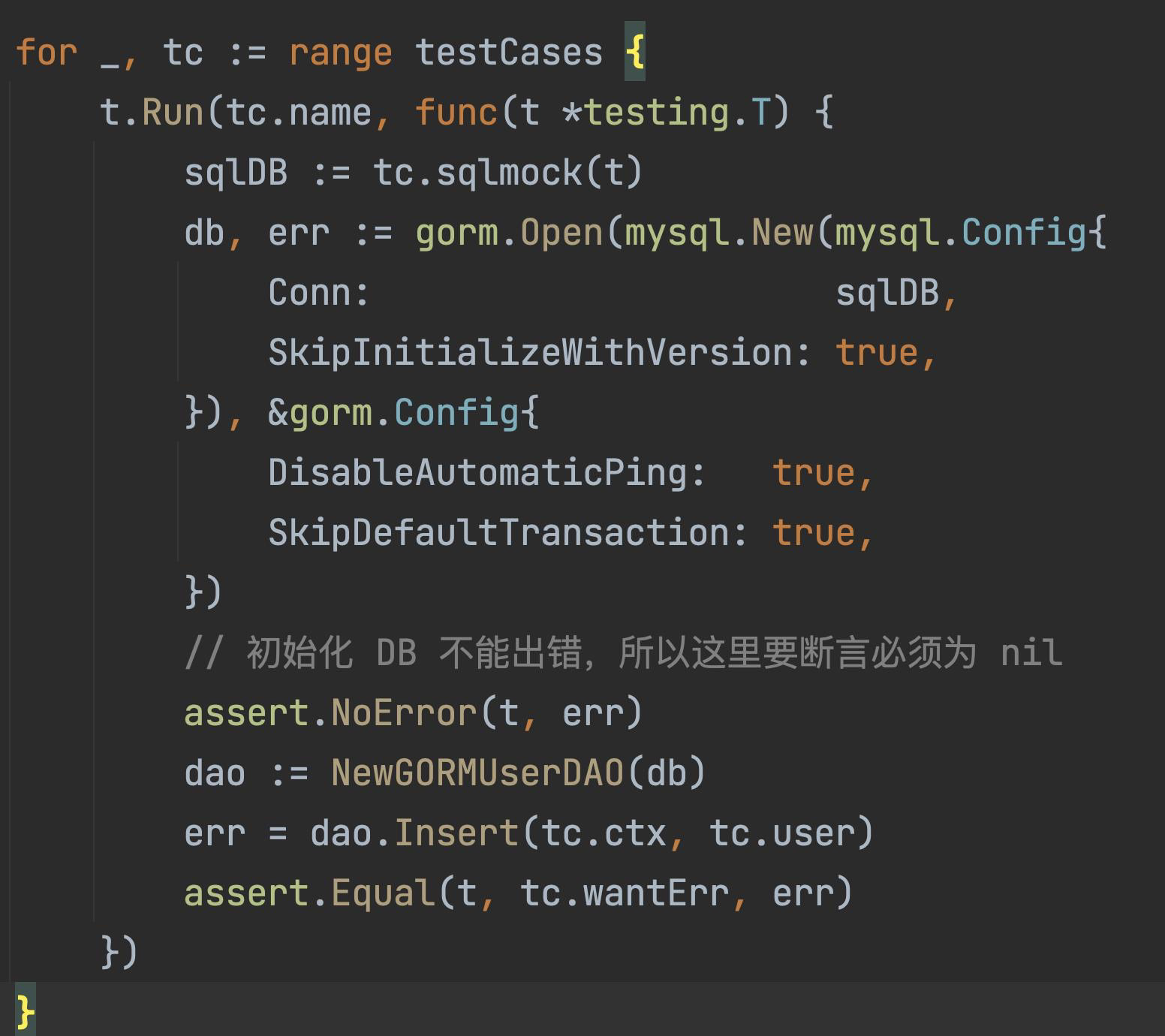
Go 单元测试之Mysql数据库集成测试
文章目录 一、 sqlmock介绍二、安装三、基本用法四、一个小案例五、Gorm 初始化注意点 一、 sqlmock介绍 sqlmock 是一个用于测试数据库交互的 Go 模拟库。它可以模拟 SQL 查询、插入、更新等操作,并且可以验证 SQL 语句的执行情况,非常适合用于单元测试…...
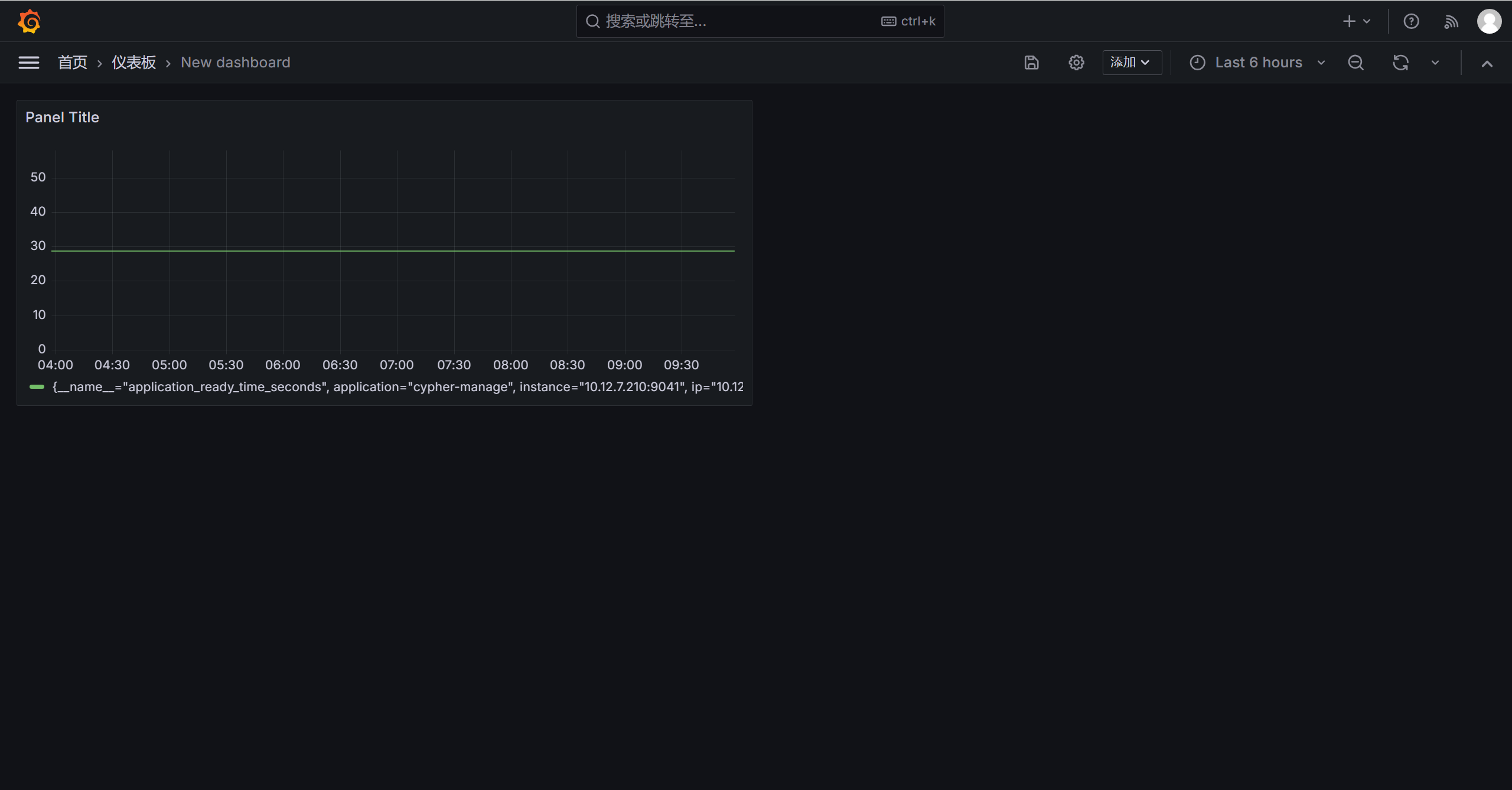
Prometheus + Grafana 搭建监控仪表盘
目标要求 1、需要展现的仪表盘: SpringBoot或JVM仪表盘 Centos物理机服务器(实际为物理分割的虚拟服务器)仪表盘 2、展现要求: 探索Prometheus Grafana搭建起来的展示效果,尽可能展示能展示的部分。 一、下载软件包 监控系统核心…...
)
机器人管理系统的增删查改(Python)
#交互模式 robot ["机器人1","机器人2","机器人3","机器人4"] name input("请输入您的姓名:") print("%s您好欢迎使用机器人管理系统"%(name))while True:print("您可以进行 1.查找 2.修改 3.增…...
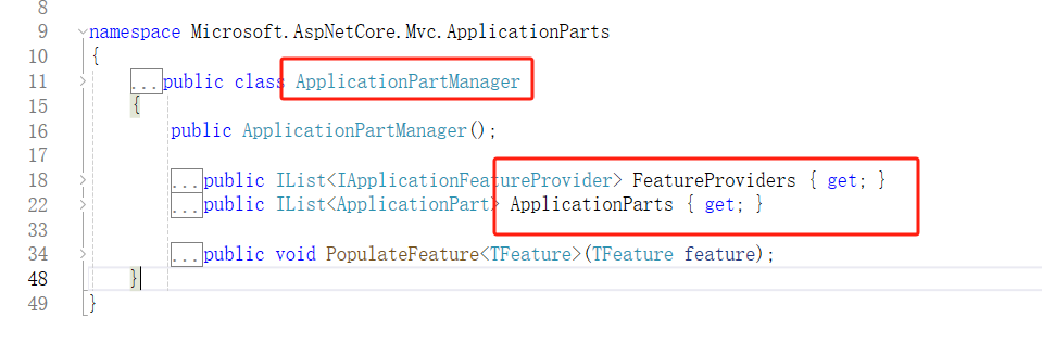
【.Net动态Web API】背景与实现原理
🚀前言 本文是《.Net Core进阶编程课程》教程专栏的导航站(点击链接,跳转到专栏主页,欢迎订阅,持续更新…) 专栏介绍:通过源码实例来讲解Asp.Net Core进阶知识点,让大家完全掌握每一…...
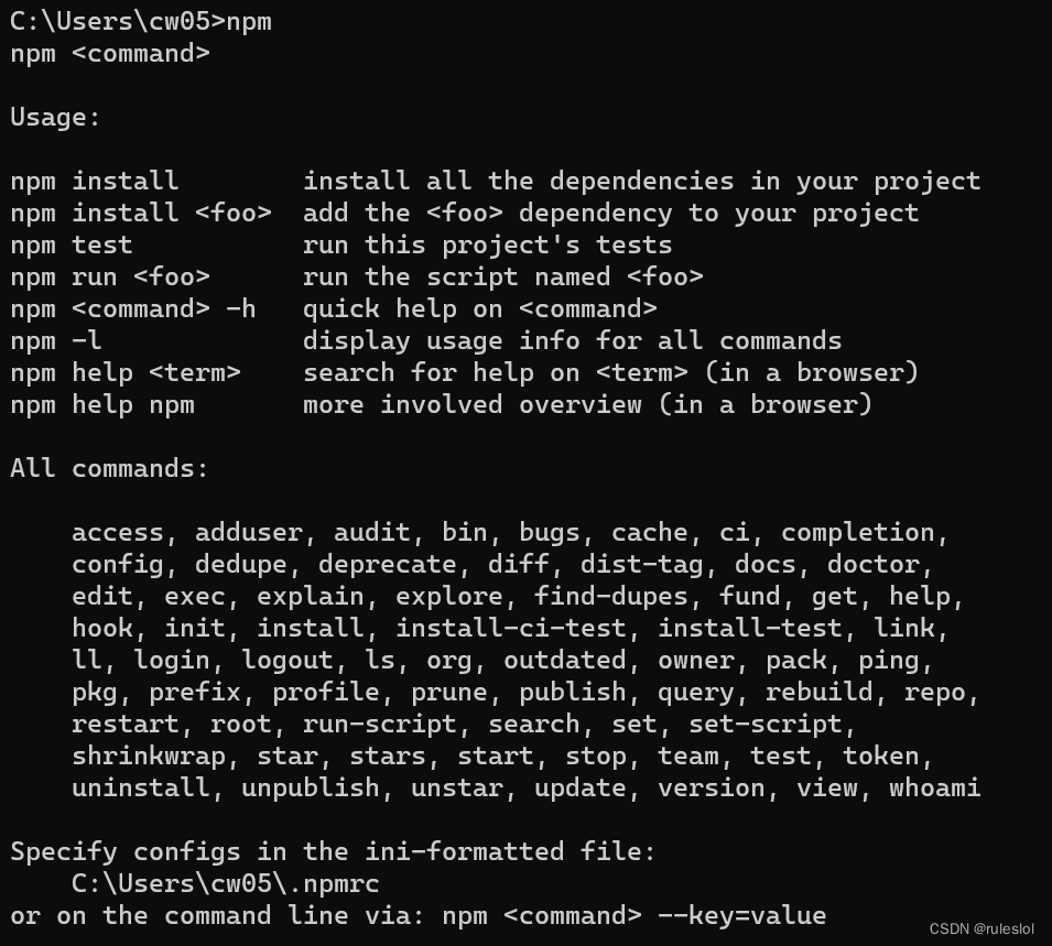
JS-43-Node.js02-安装Node.js和npm
Node.js是一个基于Chrome V8引擎的JavaScript运行时环境,可以让JavaScript实现后端开发,所以,首先在本机安装Node.js环境。 一、安装Node.js 官网:下载 Node.js 默认两个版本的下载: 64位windows系统的LTS(Long Tim…...
)
设计模式(分类)
目录 设计模式(分类) 设计模式(六大原则) 设计模式是软件工程中一种经过验证的、用于解决特定设计问题的通用解决方案。它们是面向对象编程(Object-Oriented Programming, OOP)实践中提炼出的最佳实…...

请陪伴Kimi和GPT成长
经验的闪光汤圆 但是我想要写实的 你有吗? 岁数大了,希望如何学习新知识呢?又觉得自己哪些能力亟需补强呢? 看论文自然得用Kimi,主要是肝不动了,眼睛也顶不住了。 正好昨天跟专业人士学会了用工作流的办法跟…...

优思学院|ISO45001职业健康安全管理体系是什么?
ISO45001:2018是新公布的国际标准规范,全球备受期待的职业健康与安全国际标准(OH&S)于2018年公布,并将在全球范围内改变工作场所实践。ISO45001将取代OHSAS18001,成为全球工作场所健康与安全的参考。 ISO45001:201…...

抖去推短视频矩阵系统----源头开发
为什么一直说让企业去做短视频矩阵?而好处就是有更多的流量入口,不同平台或账号之间可以进行资源互换,最终目的就是获客留咨,提单转化。你去看一些做得大的账号,你会发现他们在许多大的平台上,都有自己的账…...

Golang函数重试机制实现
前言 在编写应用程序时,有时候会遇到一些短暂的错误,例如网络请求、服务链接终端失败等,这些错误可能导致函数执行失败。 但是如果稍后执行可能会成功,那么在一些业务场景下就需要重试了,重试的概念很简单,…...
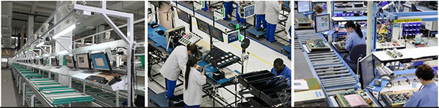
工业电脑在ESOP工作站行业应用
ESOP工作站行业应用 项目背景 E-SOP是实现作业指导书电子化,并统一管理和集中控制的一套管理信息平台。信迈科技的ESOP终端是一款体积小巧功能齐全的高性价比工业电脑,上层通过网络与MES系统连接,下层连接显示器展示作业指导书。ESOP控制终…...
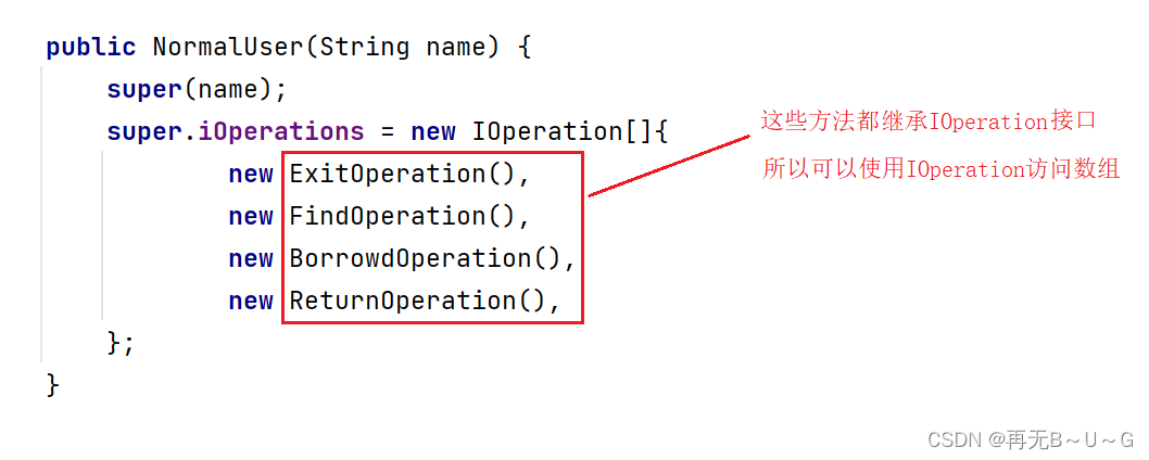
java项目实战之图书管理系统(1)
✅作者简介:大家好,我是再无B~U~G,一个想要与大家共同进步的男人😉😉 🍎个人主页:再无B~U~G-CSDN博客 1.背景 图书管理系统是一种用于管理图书…...
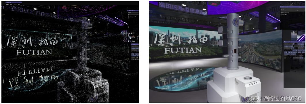
3DGS渐进式渲染 - 离线生成渲染视频
总览 输入:环绕Object拍摄的RGB视频 输出:自定义相机路径的渲染视频(包含渐变效果) 实现过程 首先,编译3DGS的C代码,并跑通convert.py、train.py和render.py。教程如下: github网址…...
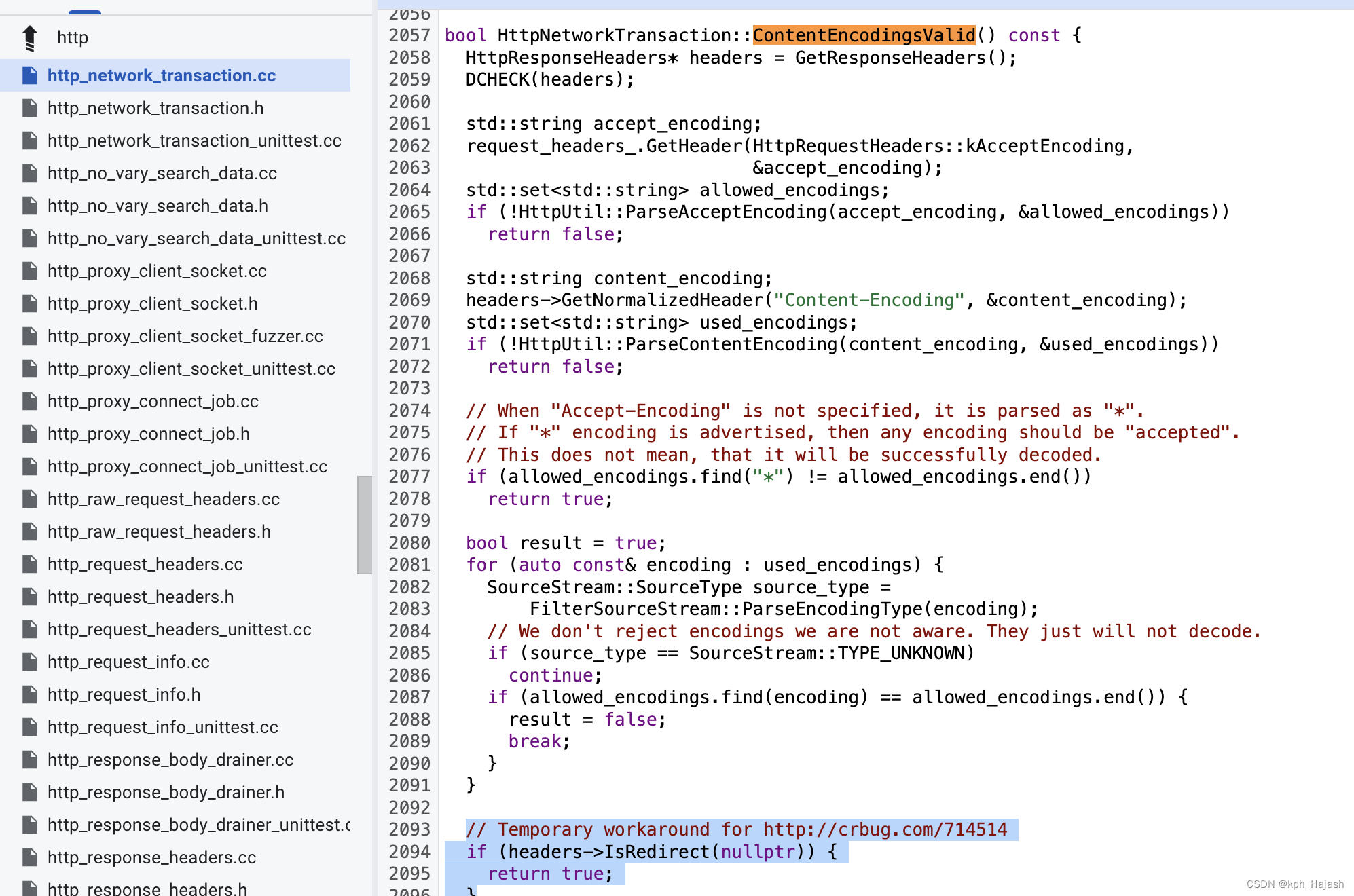
chromium 协议栈 cronet ios 踩坑案例
1、请求未携带 Accept-Language http header 出现图片加载失败 现象: 访问 https://www.huawei.com/cn/?ic_mediumdirect&ic_sourcesurlent 时出现图片加载失败的问题 预期结果: 原因: 网络库删除了添加 Accept-Language header 的逻…...
)
Java快速排序知识点(含面试大厂题和源码)
快速排序(Quick Sort)是一种高效的排序算法,采用分治法(Divide and Conquer)的策略来对一个数组进行排序。快速排序的平均时间复杂度为 O(n log n),在最坏的情况下为 O(n^2),但这种情况很少发生…...

SpringBoot整合Swagger2
SpringBoot整合Swagger2 1.什么是Swagger2?(应用场景)2.项目中如何使用2.1 导入依赖2.2 编写配置类2.3 注解使用2.3.1 controller注解:2.3.2 方法注解2.3.3 实体类注解2.3.4 方法返回值注解2.3.5 忽略的方法 3.UI界面 1.什么是Swa…...

C++算法题 - 矩阵
目录 36. 有效的数独54. 螺旋矩阵48. 旋转图像73. 矩阵置零289. 生命游戏 36. 有效的数独 LeetCode_link 请你判断一个 9 x 9 的数独是否有效。只需要 根据以下规则 ,验证已经填入的数字是否有效即可。 数字 1-9 在每一行只能出现一次。 数字 1-9 在每一列只能出现…...

记录一个没测出来,有点严重的Bug
前提: 人物:若干个 部门:若干个 部门有一个人物选择框,可以选择所有的人物,且为非必填字段 bug现象: 部门中 的人物选择框每次都少一个人物 代码分析: F12接口后端没问题,定位为前端的问题。 前…...

Oracle查询表空间大小
1 查询数据库中所有的表空间以及表空间所占空间的大小 SELECTtablespace_name,sum( bytes ) / 1024 / 1024 FROMdba_data_files GROUP BYtablespace_name; 2 Oracle查询表空间大小及每个表所占空间的大小 SELECTtablespace_name,file_id,file_name,round( bytes / ( 1024 …...
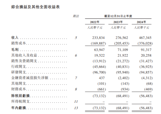
从深圳崛起的“机器之眼”:赴港乐动机器人的万亿赛道赶考路
进入2025年以来,尽管围绕人形机器人、具身智能等机器人赛道的质疑声不断,但全球市场热度依然高涨,入局者持续增加。 以国内市场为例,天眼查专业版数据显示,截至5月底,我国现存在业、存续状态的机器人相关企…...

Opencv中的addweighted函数
一.addweighted函数作用 addweighted()是OpenCV库中用于图像处理的函数,主要功能是将两个输入图像(尺寸和类型相同)按照指定的权重进行加权叠加(图像融合),并添加一个标量值&#x…...

oracle与MySQL数据库之间数据同步的技术要点
Oracle与MySQL数据库之间的数据同步是一个涉及多个技术要点的复杂任务。由于Oracle和MySQL的架构差异,它们的数据同步要求既要保持数据的准确性和一致性,又要处理好性能问题。以下是一些主要的技术要点: 数据结构差异 数据类型差异ÿ…...

C++中string流知识详解和示例
一、概览与类体系 C 提供三种基于内存字符串的流,定义在 <sstream> 中: std::istringstream:输入流,从已有字符串中读取并解析。std::ostringstream:输出流,向内部缓冲区写入内容,最终取…...
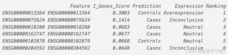
【数据分析】R版IntelliGenes用于生物标志物发现的可解释机器学习
禁止商业或二改转载,仅供自学使用,侵权必究,如需截取部分内容请后台联系作者! 文章目录 介绍流程步骤1. 输入数据2. 特征选择3. 模型训练4. I-Genes 评分计算5. 输出结果 IntelliGenesR 安装包1. 特征选择2. 模型训练和评估3. I-Genes 评分计…...

MySQL JOIN 表过多的优化思路
当 MySQL 查询涉及大量表 JOIN 时,性能会显著下降。以下是优化思路和简易实现方法: 一、核心优化思路 减少 JOIN 数量 数据冗余:添加必要的冗余字段(如订单表直接存储用户名)合并表:将频繁关联的小表合并成…...
零知开源——STM32F103RBT6驱动 ICM20948 九轴传感器及 vofa + 上位机可视化教程
STM32F1 本教程使用零知标准板(STM32F103RBT6)通过I2C驱动ICM20948九轴传感器,实现姿态解算,并通过串口将数据实时发送至VOFA上位机进行3D可视化。代码基于开源库修改优化,适合嵌入式及物联网开发者。在基础驱动上新增…...

LCTF液晶可调谐滤波器在多光谱相机捕捉无人机目标检测中的作用
中达瑞和自2005年成立以来,一直在光谱成像领域深度钻研和发展,始终致力于研发高性能、高可靠性的光谱成像相机,为科研院校提供更优的产品和服务。在《低空背景下无人机目标的光谱特征研究及目标检测应用》这篇论文中提到中达瑞和 LCTF 作为多…...

pycharm 设置环境出错
pycharm 设置环境出错 pycharm 新建项目,设置虚拟环境,出错 pycharm 出错 Cannot open Local Failed to start [powershell.exe, -NoExit, -ExecutionPolicy, Bypass, -File, C:\Program Files\JetBrains\PyCharm 2024.1.3\plugins\terminal\shell-int…...