PySpark特征工程(III)--特征选择
有这么一句话在业界广泛流传:数据和特征决定了机器学习的上限,而模型和算法只是逼近这个上限而已。由此可见,特征工程在机器学习中占有相当重要的地位。在实际应用当中,可以说特征工程是机器学习成功的关键。
特征工程是数据分析中最耗时间和精力的一部分工作,它不像算法和模型那样是确定的步骤,更多是工程上的经验和权衡。因此没有统一的方法。这里只是对一些常用的方法做一个总结。
特征工程包含了 Data PreProcessing(数据预处理)、Feature Extraction(特征提取)、Feature Selection(特征选择)和 Feature construction(特征构造)等子问题。
特征选择
现在我们已经有大量的特征可使用,有的特征携带的信息丰富,有的特征携带的信息有重叠,有的特征则属于无关特征,尽管在拟合一个模型之前很难说哪些特征是重要的,但如果所有特征不经筛选地全部作为训练特征,经常会出现维度灾难问题,甚至会降低模型的泛化性能(因为较无益的特征会淹没那些更重要的特征)。因此,我们需要进行特征筛选,排除无效/冗余的特征,把有用的特征挑选出来作为模型的训练数据。
特征选择方法有很多,一般分为三类:
- 过滤法(Filter)比较简单,它按照特征的发散性或者相关性指标对各个特征进行评分,设定评分阈值或者待选择阈值的个数,选择合适特征。
- 包装法(Wrapper)根据目标函数,通常是预测效果评分,每次选择部分特征,或者排除部分特征。
- 嵌入法(Embedded)则稍微复杂一点,它先使用选择的算法进行训练,得到各个特征的权重,根据权重从大到小来选择特征。
from pyspark.conf import SparkConf
from pyspark.sql import SparkSession
from pyspark.ml import Pipeline
from pyspark.ml import Estimator, Transformer
from pyspark.ml.feature import StringIndexer, VectorAssembler, OneHotEncoder
import pyspark.sql.functions as fn
import pyspark.ml.feature as ft
from pyspark.ml.evaluation import BinaryClassificationEvaluator, MulticlassClassificationEvaluator
from pyspark.ml.linalg import Vectors
from pyspark.sql import Row
from pyspark.sql import Observation
from pyspark.sql import Window
from pyspark.ml.tuning import CrossValidator, ParamGridBuilder, TrainValidationSplit
from xgboost.spark import SparkXGBClassifier
import xgboost as xgbimport os
import pandas as pd
import numpy as np
import matplotlib.pyplot as plt
import seaborn as snsimport time
import warnings
import gc# Setting configuration.
warnings.filterwarnings('ignore')
SEED = 42# Use 0.11.4-spark3.3 version for Spark3.3 and 1.0.2 version for Spark3.4
spark = SparkSession.builder \.master("local[*]") \.appName("XGBoost with PySpark") \.config("spark.driver.memory", "10g") \.config("spark.driver.cores", "2") \.config("spark.executor.memory", "10g") \.config("spark.executor.cores", "2") \.enableHiveSupport() \.getOrCreate()
sc = spark.sparkContext
sc.setLogLevel('ERROR')
24/06/03 21:40:26 WARN Utils: Your hostname, MacBook-Air resolves to a loopback address: 127.0.0.1; using 192.168.1.5 instead (on interface en0)
24/06/03 21:40:26 WARN Utils: Set SPARK_LOCAL_IP if you need to bind to another address
Setting default log level to "WARN".
To adjust logging level use sc.setLogLevel(newLevel). For SparkR, use setLogLevel(newLevel).
24/06/03 21:40:26 WARN NativeCodeLoader: Unable to load native-hadoop library for your platform... using builtin-java classes where applicable
定义数据集评估函数
def timer(func):import timeimport functoolsdef strfdelta(tdelta, fmt):hours, remainder = divmod(tdelta, 3600)minutes, seconds = divmod(remainder, 60)return fmt.format(hours, minutes, seconds)@functools.wraps(func)def wrapper(*args, **kwargs):click = time.time()print("Starting time\t", time.strftime("%H:%M:%S", time.localtime()))result = func(*args, **kwargs)delta = strfdelta(time.time() - click, "{:.0f} hours {:.0f} minutes {:.0f} seconds")print(f"{func.__name__} cost {delta}")return resultreturn wrapperdef progress(percent=0, width=50, desc="Processing"):import mathtags = math.ceil(width * percent) * "#"print(f"\r{desc}: [{tags:-<{width}}]{percent:.1%}", end="", flush=True)def cross_val_score(df, estimator, evaluator, features, numFolds=3, seed=SEED):df = df.withColumn('fold', (fn.rand(seed) * numFolds).cast('int'))eval_result = []# Initialize an empty dataframe to hold feature importancesfeature_importances = pd.DataFrame(index=features)for i in range(numFolds):train = df.filter(df['fold'] == i)valid = df.filter(df['fold'] != i)model = estimator.fit(train)train_pred = model.transform(train)valid_pred = model.transform(valid)train_score = evaluator.evaluate(train_pred)valid_score = evaluator.evaluate(valid_pred)metric = evaluator.getMetricName()print(f"[{i}] train's {metric}: {train_score},  valid's {metric}: {valid_score}")eval_result.append(valid_score)fscore = model.get_feature_importances()fscore = {name:fscore.get(f'f{k}', 0) for k,name in enumerate(features)}feature_importances[f'cv_{i}'] = fscorefeature_importances['fscore'] = feature_importances.mean(axis=1)return eval_result, feature_importances.sort_values('fscore', ascending=False)@timer
def score_dataset(df, inputCols=None, featuresCol=None, labelCol='label', nfold=3):assert inputCols is not None or featuresCol is not Noneif featuresCol is None:# Assemble the feature columns into a single vector columnfeaturesCol = "features"assembler = VectorAssembler(inputCols=inputCols,outputCol=featuresCol)df = assembler.transform(df)# Create an Estimator.classifier = SparkXGBClassifier(features_col=featuresCol, label_col=labelCol,eval_metric='auc',scale_pos_weight=11,learning_rate=0.015,max_depth=8,subsample=1.0,colsample_bytree=0.35,reg_alpha=65,reg_lambda=15,n_estimators=500,verbosity=0) evaluator = BinaryClassificationEvaluator(labelCol=labelCol, metricName='areaUnderROC')# Training with 3-fold CV:scores, feature_importances = cross_val_score(df=df,estimator=classifier, evaluator=evaluator,features=inputCols,numFolds=nfold)print(f"cv_agg's valid auc: {np.mean(scores):.4f} +/- {np.std(scores):.5f}")return feature_importances
df = spark.sql("select * from home_credit_default_risk.created_data")
Loading class `com.mysql.jdbc.Driver'. This is deprecated. The new driver class is `com.mysql.cj.jdbc.Driver'. The driver is automatically registered via the SPI and manual loading of the driver class is generally unnecessary.
# Persists the data in the disk by specifying the storage level.
from pyspark.storagelevel import StorageLevel
_ = df.persist(StorageLevel.MEMORY_AND_DISK)
features = df.drop('SK_ID_CURR', 'label').columns
feature_importances = score_dataset(df, inputCols=features)
Starting time	 21:40:31
[0] train's areaUnderROC: 0.8790646375204176,  valid's areaUnderROC: 0.7621647570277277
[1] train's areaUnderROC: 0.8746030416668324,  valid's areaUnderROC: 0.7576869026346968
[2] train's areaUnderROC: 0.8784984656392806,  valid's areaUnderROC: 0.7583365874350807
cv_agg's valid auc: 0.7594 +/- 0.00198
score_dataset cost 0 hours 7 minutes 33 seconds
单变量特征选择
Relief(Relevant Features)是著名的过滤式特征选择方法。该方法假设特征子集的重要性是由子集中的每个特征所对应的相关统计量分量之和所决定的。所以只需要选择前k个大的相关统计量对应的特征,或者大于某个阈值的相关统计量对应的特征即可。
| pyspark.ml.feature | |
|---|---|
| ChiSqSelector(numTopFeatures, …) | 选择用于预测分类标签的分类特征 |
| VarianceThresholdSelector(featuresCol, …) | 删除所有低方差特征 |
| UnivariateFeatureSelector(featuresCol, …) | 单变量特征选择 |
UnivariateFeatureSelector在具有分类/连续特征的分类/回归任务上选择特征。Spark根据指定的featureType和labelType参数选择要使用的评分函数。
| featureType | labelType | score function |
|---|---|---|
| categorical | categorical | chi-squared (chi2) |
| continuous | categorical | ANOVATest (f_classif) |
| continuous | continuous | F-value (f_regression) |
它支持五种选择模式:
- numTopFeatures 选择评分最高的固定数量的特征。
- percentile 选择评分最高的固定百分比的特征。
- fpr选择p值低于阈值的所有特征,从而控制假阳性选择率。
- fdr使用Benjamini-Hochberg程序来选择错误发现率低于阈值的所有特征。
- fwe选择p值低于阈值的所有功能。阈值按1/numFeatures缩放,从而控制family-wise的错误率。
如何通俗地理解Family-wise error rate(FWER)和False discovery rate(FDR)
相关系数
皮尔森相关系数是一种最简单的方法,能帮助理解两个连续变量之间的线性相关性。
定义进度条
class DropCorrelatedFeatures(Estimator, Transformer):def __init__(self, inputCols, threshold=0.9):self.inputCols = inputColsself.threshold = threshold@timerdef _fit(self, df):inputCols = [col for col,dtype in df.dtypes if dtype not in ['string', 'vector']]to_keep = [inputCols[0]]to_drop = []for c1 in inputCols[1:]:# The correlationscorr = df.select(*[fn.corr(c1, c2) for c2 in to_keep]).toPandas()# Select columns with correlations above thresholdif np.any(corr.abs().gt(self.threshold)):to_drop.append(c1)else:to_keep.append(c1)self.to_drop = to_dropself.to_keep = to_keepreturn selfdef _transform(self, df):return df.drop(*self.to_drop)
# Drops features that are correlated
# model = DropCorrelatedFeatures(features, threshold=0.9).fit(df)
# correlated = model.to_drop# print(f'Dropped {len(correlated)} correlated features.')
上述函数速度较慢,最终选择使用spark自带的相关系数矩阵:
from pyspark.ml.stat import Correlationdef drop_correlated_features(df, threshold=0.9):inputCols = [col for col,dtype in df.dtypes if dtype not in ['string', 'vector']]# Assemble the feature columns into a single vector columnassembler = VectorAssembler(inputCols=inputCols,outputCol="numericFeatures")df = assembler.transform(df)# Compute the correlation matrix with specified method using dataset.corrmat = Correlation.corr(df, 'numericFeatures', 'pearson').collect()[0][0]corrmat = pd.DataFrame(corrmat.toArray(), index=inputCols, columns=inputCols)# Upper triangle of correlationsupper = corrmat.where(np.triu(np.ones(corrmat.shape), k=1).astype('bool'))# Absolute value correlationcorr = upper.unstack().dropna().abs()to_drop = corr[corr.gt(threshold)].reset_index()['level_1'].unique()return to_drop.tolist()
correlated = drop_correlated_features(df.select(features))
selected_features = [col for col in features if col not in correlated]
print(f'Dropped {len(correlated)} correlated features.')
Dropped 127 correlated features.
卡方检验
卡方检验是一种用于衡量两个分类变量之间相关性的统计方法。
# Find categorical features
int_features = [k for k,v in df.select(selected_features).dtypes if v == 'int']
vector_features = [k for k,v in df.select(selected_features).dtypes if v == 'vector']
nunique = df.select([fn.countDistinct(var).alias(var) for var in int_features]).first().asDict()categorical_cols = [f for f, n in nunique.items() if n <= 50]
continuous_cols = list(set(selected_features) - set(categorical_cols + vector_features))
from pyspark.ml.feature import UnivariateFeatureSelectordef chi2_test_selector(df, categoricalFeatures, outputCol):selector = UnivariateFeatureSelector(featuresCol="categoricalFeatures", labelCol="label", outputCol=outputCol,selectionMode="fdr")selector.setFeatureType("categorical").setLabelType("categorical").setSelectionThreshold(0.05)# Assemble the feature columns into a single vector columnassembler = VectorAssembler(inputCols=categoricalFeatures,outputCol="categoricalFeatures")df = assembler.transform(df)model = selector.fit(df)df = model.transform(df)n = df.first()["categoricalFeatures"].sizeprint("The number of dropped features:", n - len(model.selectedFeatures))return dfdf_chi2_test = chi2_test_selector(df, categorical_cols + vector_features, 'selectedFeatures1')
The number of dropped features: 32
方差分析
方差分析主要用于分类问题中连续特征的相关性。
如果针对分类问题,方差分析和卡方检验搭配使用,就能够完成一次完整的特征筛选,其中方差分析用于筛选连续特征,卡方检验用于筛选离散特征。
def anova_selector(df, continuousFeatures, outputCol):selector = UnivariateFeatureSelector(featuresCol="continuousFeatures", labelCol="label", outputCol=outputCol,selectionMode="fdr")selector.setFeatureType("continuous").setLabelType("categorical").setSelectionThreshold(0.05)# Assemble the feature columns into a single vector columnassembler = VectorAssembler(inputCols=continuousFeatures,outputCol="continuousFeatures")df = assembler.transform(df)model = selector.fit(df)df = model.transform(df)print("The number of dropped features:", len(continuousFeatures) - len(model.selectedFeatures))return df df_anova = anova_selector(df_chi2_test, continuous_cols, 'selectedFeatures2')
The number of dropped features: 30
_ = score_dataset(df_anova, inputCols=["selectedFeatures1", "selectedFeatures2"], nfold=2)
Starting time	 21:49:20
[0] train's areaUnderROC: 0.8526299026274513,  valid's areaUnderROC: 0.7632345170337489
[1] train's areaUnderROC: 0.8533149455907856,  valid's areaUnderROC: 0.757047527015275
cv_agg's valid auc: 0.7601 +/- 0.00309
score_dataset cost 0 hours 4 minutes 16 seconds
del df_chi2_test, df_anova
gc.collect()
671
互信息
互信息是从信息熵的角度分析各个特征和目标之间的关系(包括线性和非线性关系)。
@timer
def calc_mi_scores(df, inputCols, labelCol):mi_scores = pd.Series(name="MI Scores")n = df.count()y = labelColfor x in inputCols:grouped = df.groupBy(x, y).agg(fn.count("*").alias("Num_xy")).toPandas()grouped["Num_x"] = grouped.groupby(x)["Num_xy"].transform("sum")grouped["Num_y"] = grouped.groupby(y)["Num_xy"].transform("sum")grouped["MI"] = grouped["Num_xy"] / n * np.log(grouped["Num_xy"] / grouped["Num_x"] * n / grouped["Num_y"])grouped["MI"] = grouped["MI"].where(grouped["MI"] > 0, 0)mi_scores[x] = grouped["MI"].sum()mi_scores = mi_scores.sort_values(ascending=False)return mi_scores
上述代码中采用了离散变量的互信息计算方法,在此我们先将连续变量离散化。
numBins = 50
buckets = {f"{col}_binned": col for col in continuous_cols}
bucketizer = ft.QuantileDiscretizer(numBuckets=numBins,handleInvalid='keep',inputCols=continuous_cols, outputCols=list(buckets)
).fit(df)
df = bucketizer.transform(df)discrete_cols = categorical_cols + list(buckets)
class DropUninformative(Estimator, Transformer):def __init__(self, inputCols, labelCol="label", threshold=0.0):self.threshold = thresholdself.inputCols = inputCols self.labelCol = labelColdef _fit(self, df):mi_scores = calc_mi_scores(df, self.inputCols, self.labelCol)self.to_keep = mi_scores[mi_scores > self.threshold].index.tolist()self.to_drop = list(set(self.inputCols) - set(self.to_keep))return selfdef _transform(self, df): return df.drop(*self.to_drop)
model = DropUninformative(discrete_cols, "label", threshold=0.0).fit(df)
uninformative = [buckets.get(col, col) for col in model.to_drop]print('The number of selected features:', len(model.to_keep))
print(f'Dropped {len(uninformative)} uninformative features.')
Starting time	 21:54:53
calc_mi_scores cost 0 hours 7 minutes 10 seconds
The number of selected features: 229
Dropped 5 uninformative features.
IV值
IV(Information Value)用来评价离散特征对二分类变量的预测能力。一般认为IV小于0.02的特征为无用特征。
@timer
def calc_iv_scores(df, inputCols, labelCol="label"):assert df.select(labelCol).distinct().count() == 2, "y must be binary"iv_scores = pd.Series()# Compute information valuefor var in inputCols:grouped = df.groupBy(var).agg(fn.sum(labelCol).alias('Positive'),fn.count('*').alias('All')).toPandas().set_index(var) grouped['Negative'] = grouped['All']-grouped['Positive'] grouped['Positive rate'] = grouped['Positive']/grouped['Positive'].sum()grouped['Negative rate'] = grouped['Negative']/grouped['Negative'].sum()grouped['woe'] = np.log(grouped['Positive rate']/grouped['Negative rate'])grouped['iv'] = (grouped['Positive rate']-grouped['Negative rate'])*grouped['woe']iv_scores[var] = grouped['iv'].sum()return iv_scores.sort_values(ascending=False)iv_scores = calc_iv_scores(df, discrete_cols)
print(f"There are {iv_scores.le(0.02).sum()} features with iv <=0.02.")
Starting time	 22:02:03
calc_iv_scores cost 0 hours 6 minutes 38 seconds
There are 98 features with iv <=0.02.
基尼系数
基尼系数用来衡量分类问题中特征对目标变量的影响程度。它的取值范围在0到1之间,值越大表示特征对目标变量的影响越大。常见的基尼系数阈值为0.02,如果基尼系数小于此阈值,则被认为是不重要的特征。
@timer
def calc_gini_scores(df, inputCols, labelCol="label"):gini_scores = pd.Series()# Compute gini scorefor var in inputCols:p = df.groupBy(var).agg(fn.mean(labelCol).alias("mean")).toPandas()gini = 1 - p['mean'].pow(2).sum()gini_scores[var] = gini    return gini_scores.sort_values(ascending=False)gini_scores = calc_gini_scores(df, discrete_cols)
print(f"There are {gini_scores.le(0.02).sum()} features with gini <=0.02.")
Starting time	 22:08:41
calc_gini_scores cost 0 hours 7 minutes 41 seconds
There are 1 features with gini <=0.02.
VIF值
VIF用于衡量特征之间的共线性程度。通常,VIF小于5被认为不存在多重共线性问题,VIF大于10则存在明显的多重共线性问题。
def calc_vif_scores(df):pass# vif_scores = calc_vif_scores(df)
# print(f"There are {vif_scores.gt(10).sum()} collinear features (VIF above 10)")
小结
最终,我们选择删除高相关特征和无信息特征。
features_to_drop = list(set(uninformative) | set(correlated))
selected_features = [col for col in features if col not in features_to_drop]print('The number of selected features:', len(selected_features))
print(f'Dropped {len(features_to_drop)} features.')
The number of selected features: 239
Dropped 132 features.
在371个总特征中只保留了239个,表明我们创建的许多特征是多余的。
递归消除特征
最常用的包装法是递归消除特征法(recursive feature elimination)。递归消除特征法使用一个机器学习模型来进行多轮训练,每轮训练后,消除最不重要的特征,再基于新的特征集进行下一轮训练。
由于RFE需要消耗大量的资源,这里就不编写函数运行了。
特征重要性
嵌入法也是用模型来选择特征,但是它和RFE的区别是它不通过不停的筛掉特征来进行训练,而是使用特征全集训练模型。
- 最常用的是使用带惩罚项( ℓ 1 , ℓ 2 \ell_1,\ell_2 ℓ1,ℓ2 正则项)的基模型,来选择特征,例如 Lasso,Ridge。
- 或者简单的训练基模型,选择权重较高的特征。
我们先使用之前定义的 score_dataset 获取每个特征的重要性分数:
feature_importances = score_dataset(df, inputCols=selected_features, nfold=2)
Starting time	 22:16:22
[0] train's areaUnderROC: 0.8545613660810463,  valid's areaUnderROC: 0.7633448519087491
[1] train's areaUnderROC: 0.8553078656308732,  valid's areaUnderROC: 0.7570120756115536
cv_agg's valid auc: 0.7602 +/- 0.00317
score_dataset cost 0 hours 4 minutes 24 seconds
# Sort features according to importance
feature_importances = feature_importances.sort_values('fscore', ascending=False)
feature_importances['fscore'].head(15)
AMT_GOODS_PRICE/AMT_ANNUITY       1448.0
DEF_60_CNT_SOCIAL_CIRCLE          1061.0
AMT_GOODS_PRICE/AMT_CREDIT         924.0
ln(EXT_SOURCE_2)                   867.0
ln(EXT_SOURCE_3)                   793.5
ORGANIZATION_TYPE/DAYS_BIRTH       777.5
DAYS_BIRTH/EXT_SOURCE_1            776.5
EXT_SOURCE_3/ORGANIZATION_TYPE     723.0
EXT_SOURCE_3/DAYS_BIRTH            687.5
ORGANIZATION_TYPE/EXT_SOURCE_1     685.5
centroid_0                         662.5
EXT_SOURCE_2/ORGANIZATION_TYPE     658.5
EXT_SOURCE_2/DAYS_BIRTH            635.0
AMT_ANNUITY/AMT_INCOME_TOTAL       622.5
EXT_SOURCE_1/DAYS_BIRTH            587.0
Name: fscore, dtype: float64
可以看到,我们构建的许多特征进入了前15名,这应该让我们有信心,我们所有的辛勤工作都是值得的!
接下来,我们删除重要性为0的特征,因为这些特征实际上从未用于在任何决策树中拆分节点。因此,删除这些特征是一个非常安全的选择(至少对这个特定模型来说)。
# Find the features with zero importance
zero_importance = feature_importances.query("fscore == 0.0").index.tolist()
print(f'\nThere are {len(zero_importance)} features with 0.0 importance')
There are 7 features with 0.0 importance
selected_features = [col for col in selected_features if col not in zero_importance]
print("The number of selected features:", len(selected_features))
print("Dropped {} features with zero importance.".format(len(zero_importance)))
The number of selected features: 232
Dropped 7 features with zero importance.
删除0重要性的特征后,我们还有232个特征。如果我们认为此时特征量依然非常大,我们可以继续删除重要性最小的特征。
下图显示了累积重要性与特征数量:
feature_importances = feature_importances.sort_values('fscore', ascending=False)sns.lineplot(x=range(1, feature_importances.shape[0]+1), y=feature_importances['fscore'].cumsum())
plt.show()

如果我们选择是只保留95%的重要性所需的特征:
def select_import_features(scores, thresh=0.95):feature_imp = pd.DataFrame({'score': feature_importances['fscore']})# Sort features according to importancefeature_imp = feature_imp.sort_values('score', ascending=False)# Normalize the feature importancesfeature_imp['score_normalized'] = feature_imp['score'] / feature_imp['score'].sum()feature_imp['cumsum'] = feature_imp['score_normalized'].cumsum()selected_features = feature_imp.query(f'cumsum <= {thresh}')return selected_features.index.tolist()import_features = select_import_features(feature_importances['fscore'], thresh=0.95)
print("The number of import features:", len(import_features))
print(f'Dropped {len(selected_features) - len(import_features)} features.')
The number of import features: 157
Dropped 75 features.
剩余157个特征足以覆盖95%的重要性。
feature_importances = score_dataset(df, inputCols=import_features)
Starting time	 22:20:46
[0] train's areaUnderROC: 0.8645996680043095,  valid's areaUnderROC: 0.7537419087196509
[1] train's areaUnderROC: 0.8617688316741262,  valid's areaUnderROC: 0.7494887919280331
[2] train's areaUnderROC: 0.8602027702822611,  valid's areaUnderROC: 0.7489103752356694
cv_agg's valid auc: 0.7507 +/- 0.00215
score_dataset cost 0 hours 3 minutes 58 seconds
在继续之前,我们应该记录我们采取的特征选择步骤,以备将来使用:
- 删除互信息为0的无效特征:删除了5个特征
- 删除相关系数大于0.9的共线变量:删除了127个特征
- 根据GBM删除0.0重要特征:删除7个特征
- (可选)仅保留95%特征重要性所需的特征:删除了75个特征
我们看下特征组成:
original_df = spark.sql("select * from home_credit_default_risk.prepared_data").limit(1).toPandas()original_features = [f for f in selected_features if f in original_df.columns]
derived_features =  [f for f in selected_features if f not in original_features]print(f"Selected features: {len(original)} original features, {len(derived)} derived features.")
Selected features: 79 original features, 153 derived features.
保留的222个特征,有79个是原始特征,153个是衍生特征。
主成分分析
常见的降维方法除了基于L1惩罚项的模型以外,另外还有主成分分析法(PCA)和线性判别分析(LDA)。这两种方法的本质是相似的,本节主要介绍PCA。
pca = ft.PCA(k=len(features), inputCol="scaled", outputCol="pcaFeatures"
)
# Assemble the feature columns into a single vector column
assembler = VectorAssembler(inputCols=features,outputCol="features"
)
scaler = ft.RobustScaler(inputCol="features",outputCol="scaled"
)pipeline = Pipeline(stages=[assembler, scaler, pca]).fit(df)
pcaModel = pipeline.stages[2]
print("explained variance ratio:\n", pcaModel.explainedVariance[:5])pca_df = pipeline.transform(df)
weight_matrix = pcaModel.pc
explained variance ratio:[9.47148918e-01 4.88162534e-02 3.38563499e-03 2.82225779e-047.15668020e-05]
其中 pcaModel.pc 对应 PCA 求解矩阵的SVD分解的截断矩阵 V V V,形状为 (n_features, n_components) ,其中 n_components 是我们指定的主成分数目,n_features 是原始数据的特征数目。pcaModel.pc 的每一列表示一个主成分,每一行表示原始数据的一个特征。因此,pca.components_ 的每个元素表示对应特征在主成分中的权重。
可视化方差
def plot_variance(pca, n_components=10):evr = pca.explainedVariance[:n_components]grid = range(1, n_components + 1)# Create figureplt.figure(figsize=(6, 4))# Percentage of variance explained for each components.plt.bar(grid, evr, label='Explained Variance')# Cumulative Varianceplt.plot(grid, np.cumsum(evr), "o-", label='Cumulative Variance', color='orange')  plt.xlabel("The number of Components")plt.xticks(grid)plt.title("Explained Variance Ratio")plt.ylim(0.0, 1.1)plt.legend(loc='best')plot_variance(pcaModel)
plt.show()

PCA可以有效地减少维度的数量,但他们的本质是要将原始的样本映射到维度更低的样本空间中。这意味着PCA特征没有真正的业务含义。此外,PCA假设数据是正态分布的,这可能不是真实数据的有效假设。因此,我们只是展示了如何使用pca,实际上并没有将其应用于数据。
总结
本章介绍了很多特征选择方法
- 单变量特征选择可以用于理解数据、数据的结构、特点,也可以用于排除不相关特征,但是它不能发现冗余特征。
- 正则化的线性模型可用于特征理解和特征选择。但是它需要先把特征转换成正态分布。
- 嵌入法的特征重要性选择是一种非常流行的特征选择方法,它易于使用。但它有两个主要问题:
- 重要的特征有可能得分很低(关联特征问题)
- 这种方法对类别多的特征越有利(偏向问题)
至此,经典的特征工程至此已经完结了,我们继续使用XGBoost模型评估筛选后的特征。
feature_importances = score_dataset(df, selected_features, nfold=2)
Starting time	 22:27:24
[0] train's areaUnderROC: 0.8514944460937176,  valid's areaUnderROC: 0.7609365503074478
[1] train's areaUnderROC: 0.8528487869720561,  valid's areaUnderROC: 0.7552742165606054
cv_agg's valid auc: 0.7581 +/- 0.00283
score_dataset cost 0 hours 4 minutes 8 seconds
特征重要性:
# Sort features according to importance
feature_importances['fscore'].sort_values(ascending=False).head(15)
AMT_GOODS_PRICE/AMT_ANNUITY       1351.0
ln(EXT_SOURCE_2)                   878.0
AMT_GOODS_PRICE/AMT_CREDIT         876.5
ORGANIZATION_TYPE/DAYS_BIRTH       840.0
EXT_SOURCE_3/DAYS_BIRTH            749.0
DAYS_BIRTH/EXT_SOURCE_1            724.5
centroid_0                         689.0
ln(EXT_SOURCE_3)                   681.0
EXT_SOURCE_2/DAYS_BIRTH            675.5
EXT_SOURCE_1/DAYS_BIRTH            670.0
EXT_SOURCE_3/ORGANIZATION_TYPE     659.5
AMT_REQ_CREDIT_BUREAU_QRT          638.0
EXT_SOURCE_2/ORGANIZATION_TYPE     635.5
AMT_ANNUITY/AMT_INCOME_TOTAL       629.5
ORGANIZATION_TYPE/EXT_SOURCE_1     593.5
Name: fscore, dtype: float64
保存数据集
selected_data = df.select('SK_ID_CURR', 'label', *selected_features)
selected_data.write.bucketBy(100, "SK_ID_CURR").mode("overwrite").saveAsTable("home_credit_default_risk.selected_data")
spark.stop()
相关文章:
PySpark特征工程(III)--特征选择
有这么一句话在业界广泛流传:数据和特征决定了机器学习的上限,而模型和算法只是逼近这个上限而已。由此可见,特征工程在机器学习中占有相当重要的地位。在实际应用当中,可以说特征工程是机器学习成功的关键。 特征工程是数据分析…...
Mongodb的数据库简介、docker部署、操作语句以及java应用
Mongodb的数据库简介、docker部署、操作语句以及java应用 本文主要介绍了mongodb的基础概念和特点,以及基于docker的mongodb部署方法,最后介绍了mongodb的常用数据库操作语句(增删改查等)以及java下的常用语句。 一、基础概念 …...

七大战略性新兴产业崭露头角:新能源电燃灶或将成为未来厨房新宠
近日,在国家发布的七大战略性新兴产业名单中,新能源产业赫然在列,作为其中的重要组成部分,华火新能源电燃灶凭借其独特的优势,正逐渐走进人们的视野,有望成为未来厨房的新宠。 华火新能源电燃灶作为清洁能源…...

C#进阶-用于Excel处理的程序集
在.NET开发中,处理Excel文件是一项常见的任务,而有一些优秀的Excel处理包可以帮助开发人员轻松地进行Excel文件的读写、操作和生成。本文介绍了NPOI、EPPlus和Spire.XLS这三个常用的.NET Excel处理包,分别详细介绍了它们的特点、示例代码以及…...
)
持续总结中!2024年面试必问 20 道 Kafka面试题(五)
上一篇地址:持续总结中!2024年面试必问 20 道 Kafka面试题(四)-CSDN博客 九、请解释Kafka中的Zookeeper的作用。 在Kafka中,ZooKeeper扮演着至关重要的角色,主要负责集群管理、协调和状态同步等功能。以下…...

Draw.io 使用详细教程
Draw.io 是一款功能强大的在线绘图工具,适用于创建流程图、网络图、组织结构图、UML 图等。以下是详细的使用教程,包括基本操作、快捷键、常用技巧和进阶技巧。 1. 创建新图 选择存储位置 首次使用时,系统会询问你要将图保存到哪里。你可以…...
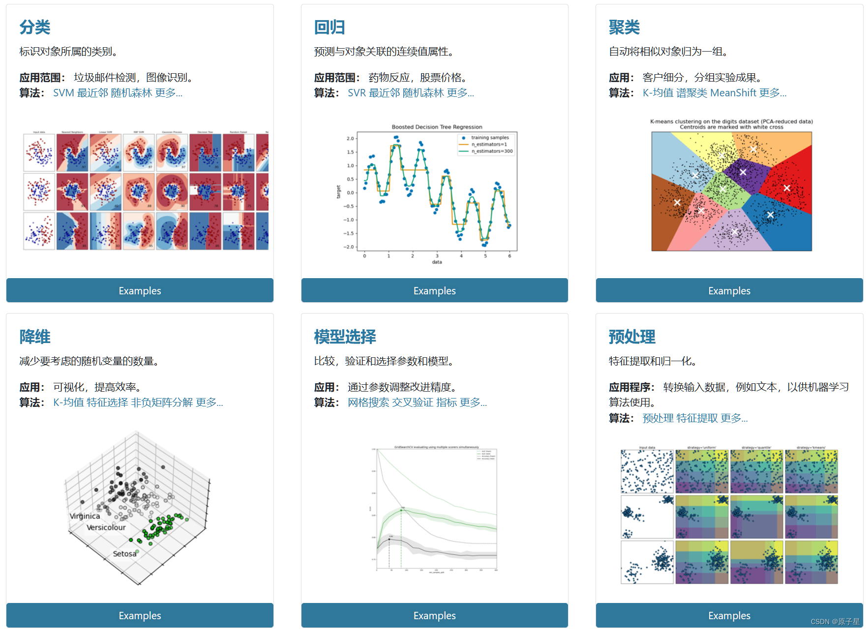
人工智能学习笔记(1):了解sklearn
sklearn 简介 Sklearn是一个基于Python语言的开源机器学习库。全称Scikit-Learn,是建立在诸如NumPy、SciPy和matplotlib等其他Python库之上,为用户提供了一系列高质量的机器学习算法,其典型特点有: 简单有效的工具进行预测数据分…...

PromptPort:为大模型定制的创意AI提示词工具库
PromptPort:为大模型定制的创意AI提示词工具库 随着人工智能技术的飞速发展,大模型在各行各业的应用越来越广泛。而在与大模型交互的过程中,如何提供精准、有效的提示词成为了关键。今天,就为大家介绍一款专为大模型定制的创意AI…...

IDEA升级web项目为maven项目乱码
今天将一个java web项目改造为maven项目。 首先,创建一个新的maven项目,将文件拷贝到新项目中。 其次,将旧项目的jar包,在maven的pom.xml做成依赖 接着,把没有maven坐标的jar包在编译的时候也包含进来 <build>…...

存内计算与扩散模型:下一代视觉AIGC能力提升的关键
目录 前言 视觉AIGC的ChatGPT4.0时代 扩散模型的算力“饥渴症” 存内计算解救算力“饥渴症” 结语 前言 在这个AI技术日新月异的时代,我们正见证着前所未有的创新与变革。尤其是在视觉内容生成领域(AIGC,Artificial Intelligence Generate…...

如何上传模型素材创建3D漫游作品?
一、进入3D空间漫游互动工具编辑器 进入720云官网-点击“开始创作”-选择3D空间漫游-进入到作品创建页面。 二、上传模型及素材,创建生成3D空间漫游模型 1.创建3D空间作品:您可以选择新建空白作品或使用720云提供的预设空间模板,本篇主要介绍…...
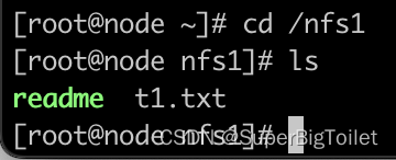
NFS p.1 服务器的部署以及客户端与服务端的远程挂载
目录 介绍 应用 NFS的工作原理 NFS的使用 步骤 1、两台机子 2、安装 3、配置文件 4、实验 服务端 准备 启动服务: 客户端 准备 步骤 介绍 NFS(Network File System,网络文件系统)是一种古老的用于在UNIX/Linux主…...
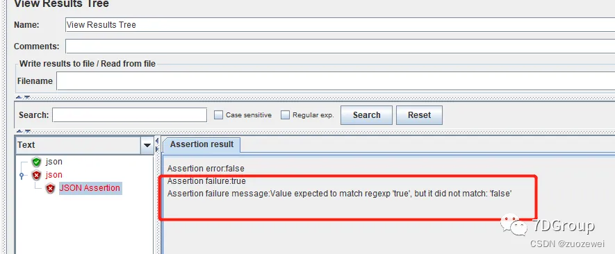
性能工具之 JMeter 常用组件介绍(二)
文章目录 一、Thread Group二、断言组件1、Response Assertion:响应断言2、Response Assertion:响应断言3、Duration Assertion:响应时间断言4.、JSON Assertion:json断言 一、Thread Group 线程组也叫用户组,是性能测…...

Bev 车道标注方案及复杂车道线解决
文章目录 1. 数据采集方案1.1 传感器方案1.2 数据同步2. 标注方案2.1 标注注意项2.2 4d 标注(时序)2.2.1 4d标签制作2.2.2 时序融合的作用2.2.2.1 时序融合方式2.2.2.2 时序融合难点2.2.2.2 时序实际应用情况3. 复杂车道线解决3.1 split 和merge车道线的解决3.2 大曲率或U形车道…...
vue 将echart 下载为base64图片
1 echart是页面的子组件, 2 页面有多个echart 3 将多个echart下载为base64图片 // 子组件 echart,要保存echartconst chart this.$echarts.init(this.$refs.chart, light) this.chartData chart; //保存数据,供父组件alarmReport调用(th…...

视频汇聚EasyCVR平台视图库GA/T 1400协议与GB/T 28181协议的区别
在公安和公共安全领域,视频图像信息的应用日益广泛,尤其是在监控、安防和应急指挥等方面。为了实现视频信息的有效传输、接收和处理,GA/T 1400和GB/T 28181这两个协议被广泛应用。虽然两者都服务于视频信息处理的目的,但它们在实际…...

白杨SEO:小红书标题怎么写?小红书怎么推广引流到微信?小红书违规注销不了怎么办?33个小红书运营常见问题解答【干货】
前言:这是白杨SEO公号原创第533篇。为什么想到写这个?因为很多白杨SEO朋友在做小红书遇到这样或那样的问题来问我,所以我把一些问得较多的常见热门问题整理写出来,有需要的可以随时查看,收藏与分享。图片在公众号白杨S…...

Linux压测
目录 CPU压测 内存压测 本文主要是编写了shell脚本,对Linux系统进行CPU和内存的压测。 CPU压测 [rootlocalhost ~]# cat cpu_stress_test.sh #!/bin/bash # 定义压测CPU的函数 function test_cpu() { # 初始化时间变量 local time # 获取参数 while geto…...
Linux如何远程连接服务器?
远程连接服务器是当代计算机技术中一个非常重要的功能,在各种领域都有广泛的应用。本文将重点介绍如何使用Linux系统进行远程连接服务器操作。 SSH协议 远程连接服务器最常用的方式是使用SSH(Secure Shell)协议。SSH是一种网络协议ÿ…...

Java 应用部署与优化:简单介绍Java应用的部署策略,并讲解一些常用的Java应用性能优化技巧
I. Java 应用部署 A. 容器化部署 Docker 的简介及其优势 Docker是一种开源的容器化技术,它可以将应用及其依赖打包在一起作为一个可运行的独立单元进行运行。Docker的主要优势包括以下几点: 便携性:无论在哪种环境下,只要安装了Docker,就可以运行Docker容器。 一致性:…...

开源抢票工具成功率提升指南:从配置到实战的全方位优化
开源抢票工具成功率提升指南:从配置到实战的全方位优化 【免费下载链接】damaihelper 支持大麦网,淘票票、缤玩岛等多个平台,演唱会演出抢票脚本 项目地址: https://gitcode.com/gh_mirrors/dam/damaihelper 你是否曾在开票瞬间眼睁睁…...

STM32 串口发送中文
一、汉字编码基础 1.1、汉字识别 UTF-8编码特点:汉字通常占3个字节;首字节特征:1110xxxx (0xE0-0xEF)(都 > 0x7F);后续字节特征:10xxxxxx (0x80-0xBF)(都 > 0x7F) …...

Ostrakon-VL-8B构建智能相册:基于自然语言的照片检索与回忆生成
Ostrakon-VL-8B构建智能相册:基于自然语言的照片检索与回忆生成 你有没有过这样的经历?手机里存了几千张照片,想找一张去年夏天在山上拍的照片,却要翻上十几分钟,甚至最后也没找到。或者,看着一堆旅行照片…...

开源工具终极方案:3步解锁Cursor Pro全功能完全指南
开源工具终极方案:3步解锁Cursor Pro全功能完全指南 【免费下载链接】cursor-free-vip [Support 0.45](Multi Language 多语言)自动注册 Cursor Ai ,自动重置机器ID , 免费升级使用Pro 功能: Youve reached your trial…...

新手福音:通过快马AI生成代码学习下拉词功能实现原理
今天想和大家分享一个特别适合前端新手练手的小项目——实现一个基础的下拉词搜索框。这个功能看似简单,但涵盖了事件监听、数组过滤、DOM操作等前端开发的核心概念。我自己在学习过程中发现,通过实际动手实现一个小功能,比单纯看理论要容易理…...

Qwen2.5-VL-7B-InstructGPU优化指南:视觉特征缓存机制与响应速度实测对比
Qwen2.5-VL-7B-Instruct GPU优化指南:视觉特征缓存机制与响应速度实测对比 1. 项目概述与优化背景 Qwen2.5-VL-7B-Instruct作为一款先进的多模态视觉-语言模型,在处理图像和文本交互任务时展现出强大能力。但在实际部署中,我们发现其GPU资源…...

HTML函数在高负载下自动关机是硬件问题吗_过热保护机制【汇总】
HTML没有函数,更不会导致关机;所谓“HTML函数关机”是误解,实际是高负载JS/渲染引发CPU/GPU过热,触发系统级温控断电。HTML 函数在高负载下自动关机?压根不存在这个函数HTML 是标记语言,没有“函数”&#…...

提升编码效率:用快马平台调用codex自动生成常用工具函数库
提升编码效率:用快马平台调用codex自动生成常用工具函数库 最近在开发一个前端项目时,发现每次都要重复写一些基础工具函数,比如日期格式化、对象深拷贝这些。虽然网上能找到现成的代码,但质量参差不齐,整合起来也很费…...

D3KeyHelper:如何通过智能操作优化解放暗黑3玩家双手的效率工具
D3KeyHelper:如何通过智能操作优化解放暗黑3玩家双手的效率工具 【免费下载链接】D3keyHelper D3KeyHelper是一个有图形界面,可自定义配置的暗黑3鼠标宏工具。 项目地址: https://gitcode.com/gh_mirrors/d3/D3keyHelper 一、问题场景:…...

Markdown 使用指南
这里写自定义目录标题欢迎使用Markdown编辑器新的改变功能快捷键合理的创建标题,有助于目录的生成如何改变文本的样式插入链接与图片如何插入一段漂亮的代码片生成一个适合你的列表创建一个表格设定内容居中、居左、居右SmartyPants创建一个自定义列表如何创建一个注…...