第100+14步 ChatGPT学习:R实现随机森林分类
基于R 4.2.2版本演示
一、写在前面
有不少大佬问做机器学习分类能不能用R语言,不想学Python咯。
答曰:可!用GPT或者Kimi转一下就得了呗。
加上最近也没啥内容写了,就帮各位搬运一下吧。
二、R代码实现随机森林分类
(1)导入数据
我习惯用RStudio自带的导入功能:


(2)建立随机森林模型(默认参数)
# Load necessary libraries
library(caret)
library(pROC)
library(ggplot2)# Assume 'data' is your dataframe containing the data
# Set seed to ensure reproducibility
set.seed(123)# Split data into training and validation sets (80% training, 20% validation)
trainIndex <- createDataPartition(data$X, p = 0.8, list = FALSE)
trainData <- data[trainIndex, ]
validData <- data[-trainIndex, ]# Convert the target variable to a factor for classification
trainData$X <- as.factor(trainData$X)
validData$X <- as.factor(validData$X)# Define control method for training with cross-validation
trainControl <- trainControl(method = "cv", number = 10)# Fit Random Forest model on the training set
model <- train(X ~ ., data = trainData, method = "rf", trControl = trainControl)# Print the best parameters found by the model
best_params <- model$bestTune
cat("The best parameters found are:\n")
print(best_params)
# Predict on the training and validation sets
trainPredict <- predict(model, trainData, type = "prob")[,2]
validPredict <- predict(model, validData, type = "prob")[,2]# Calculate ROC curves and AUC values
trainRoc <- roc(response = trainData$X, predictor = trainPredict)
validRoc <- roc(response = validData$X, predictor = validPredict)# Plot ROC curves with AUC values
ggplot(data = data.frame(fpr = trainRoc$specificities, tpr = trainRoc$sensitivities), aes(x = 1 - fpr, y = tpr)) +geom_line(color = "blue") +geom_area(alpha = 0.2, fill = "blue") +geom_abline(slope = 1, intercept = 0, linetype = "dashed", color = "black") +ggtitle("Training ROC Curve") +xlab("False Positive Rate") +ylab("True Positive Rate") +annotate("text", x = 0.5, y = 0.1, label = paste("Training AUC =", round(auc(trainRoc), 2)), hjust = 0.5, color = "blue")ggplot(data = data.frame(fpr = validRoc$specificities, tpr = validRoc$sensitivities), aes(x = 1 - fpr, y = tpr)) +geom_line(color = "red") +geom_area(alpha = 0.2, fill = "red") +geom_abline(slope = 1, intercept = 0, linetype = "dashed", color = "black") +ggtitle("Validation ROC Curve") +xlab("False Positive Rate") +ylab("True Positive Rate") +annotate("text", x = 0.5, y = 0.2, label = paste("Validation AUC =", round(auc(validRoc), 2)), hjust = 0.5, color = "red")# Calculate confusion matrices based on 0.5 cutoff for probability
confMatTrain <- table(trainData$X, trainPredict >= 0.5)
confMatValid <- table(validData$X, validPredict >= 0.5)# Function to plot confusion matrix using ggplot2
plot_confusion_matrix <- function(conf_mat, dataset_name) {conf_mat_df <- as.data.frame(as.table(conf_mat))colnames(conf_mat_df) <- c("Actual", "Predicted", "Freq")p <- ggplot(data = conf_mat_df, aes(x = Predicted, y = Actual, fill = Freq)) +geom_tile(color = "white") +geom_text(aes(label = Freq), vjust = 1.5, color = "black", size = 5) +scale_fill_gradient(low = "white", high = "steelblue") +labs(title = paste("Confusion Matrix -", dataset_name, "Set"), x = "Predicted Class", y = "Actual Class") +theme_minimal() +theme(axis.text.x = element_text(angle = 45, hjust = 1), plot.title = element_text(hjust = 0.5))print(p)
}# Now call the function to plot and display the confusion matrices
plot_confusion_matrix(confMatTrain, "Training")
plot_confusion_matrix(confMatValid, "Validation")# Extract values for calculations
a_train <- confMatTrain[1, 1]
b_train <- confMatTrain[1, 2]
c_train <- confMatTrain[2, 1]
d_train <- confMatTrain[2, 2]a_valid <- confMatValid[1, 1]
b_valid <- confMatValid[1, 2]
c_valid <- confMatValid[2, 1]
d_valid <- confMatValid[2, 2]# Training Set Metrics
acc_train <- (a_train + d_train) / sum(confMatTrain)
error_rate_train <- 1 - acc_train
sen_train <- d_train / (d_train + c_train)
sep_train <- a_train / (a_train + b_train)
precision_train <- d_train / (b_train + d_train)
F1_train <- (2 * precision_train * sen_train) / (precision_train + sen_train)
MCC_train <- (d_train * a_train - b_train * c_train) / sqrt((d_train + b_train) * (d_train + c_train) * (a_train + b_train) * (a_train + c_train))
auc_train <- roc(response = trainData$X, predictor = trainPredict)$auc# Validation Set Metrics
acc_valid <- (a_valid + d_valid) / sum(confMatValid)
error_rate_valid <- 1 - acc_valid
sen_valid <- d_valid / (d_valid + c_valid)
sep_valid <- a_valid / (a_valid + b_valid)
precision_valid <- d_valid / (b_valid + d_valid)
F1_valid <- (2 * precision_valid * sen_valid) / (precision_valid + sen_valid)
MCC_valid <- (d_valid * a_valid - b_valid * c_valid) / sqrt((d_valid + b_valid) * (d_valid + c_valid) * (a_valid + b_valid) * (a_valid + c_valid))
auc_valid <- roc(response = validData$X, predictor = validPredict)$auc# Print Metrics
cat("Training Metrics\n")
cat("Accuracy:", acc_train, "\n")
cat("Error Rate:", error_rate_train, "\n")
cat("Sensitivity:", sen_train, "\n")
cat("Specificity:", sep_train, "\n")
cat("Precision:", precision_train, "\n")
cat("F1 Score:", F1_train, "\n")
cat("MCC:", MCC_train, "\n")
cat("AUC:", auc_train, "\n\n")cat("Validation Metrics\n")
cat("Accuracy:", acc_valid, "\n")
cat("Error Rate:", error_rate_valid, "\n")
cat("Sensitivity:", sen_valid, "\n")
cat("Specificity:", sep_valid, "\n")
cat("Precision:", precision_valid, "\n")
cat("F1 Score:", F1_valid, "\n")
cat("MCC:", MCC_valid, "\n")
cat("AUC:", auc_valid, "\n")
在R语言中,使用 caret 包训练随机森林模型时,最常见的可调参数是 mtry,但还有其他几个参数可以根据需要调整。这些参数通常是从 randomForest 包继承而来的,因为 caret 包的随机森林方法默认使用的是这个包(所以第一次要安装)。下面是一些可以调整的关键参数:
①mtry: 在每个分割中考虑的变量数量。默认情况下,对于分类问题,mtry 默认值是总变量数的平方根;对于回归问题,是总变量数的三分之一。
②ntree: 构建的树的数量。更多的树可以提高模型的稳定性和准确性,但会增加计算时间和内存使用。默认值通常是 500。
③nodesize: 每个叶节点最少包含的样本数。增加这个参数的值可以减少模型的过拟合,但可能会导致欠拟合。对于分类问题,默认值通常为 1,而回归问题则较大。
④maxnodes: 最大的节点数。这限制了树的最大大小,可以用来控制模型复杂度。
⑤importance: 是否计算变量重要性。这不会影响模型的预测能力,但会影响变量重要性分数的计算。
⑥replace: 是否进行有放回抽样。默认为 TRUE,意味着进行有放回的抽样。
⑦classwt: 类的权重,用于分类问题中的不平衡数据。
⑧cutoff: 分类问题中用于预测类别的概率阈值。这通常是一个类别数目的向量。
⑨sampsize: 用于每棵树的样本大小,如果使用有放回抽样(replace=TRUE),它决定了每个样本被抽样的次数。
结果输出(默认参数):


在默认参数中,caret包只会默默帮我们找几个合适的mtry值进行测试,其他默认值。
随机森林祖传的过拟合现象。
三、随机森林调参方法(4个值)
设置mtry值取值2、数据集列数的平方根、数据集列数的一半;ntree取值100、500和1000;nodesize取值1、5、10;maxnodes取值30、50、100:
# Load necessary libraries
library(caret)
library(pROC)
library(ggplot2)
library(randomForest)  # Using randomForest for model fitting# Assume 'data' is your dataframe containing the data
# Set seed to ensure reproducibility
set.seed(123)# Split data into training and validation sets (80% training, 20% validation)
trainIndex <- createDataPartition(data$X, p = 0.8, list = FALSE)
trainData <- data[trainIndex, ]
validData <- data[-trainIndex, ]# Convert the target variable to a factor for classification
trainData$X <- as.factor(trainData$X)
validData$X <- as.factor(validData$X)# Define ranges for each parameter including mtry
mtry_range <- c(2, sqrt(ncol(trainData)), ncol(trainData)/2)
ntree_range <- c(100, 500, 1000)
nodesize_range <- c(1, 5, 10)
maxnodes_range <- c(30, 50, 100)# Initialize variables to store the best model, its AUC, and parameters
best_auc <- 0
best_model <- NULL
best_params <- NULL  # Initialize best_params to store parameter values# Nested loops to try different combinations of parameters including mtry
for (mtry in mtry_range) {for (ntree in ntree_range) {for (nodesize in nodesize_range) {for (maxnodes in maxnodes_range) {# Train the Random Forest modelrf_model <- randomForest(X ~ ., data = trainData, mtry=mtry, ntree=ntree, nodesize=nodesize, maxnodes=maxnodes)# Predict on validation set using probabilities for ROCvalidProb <- predict(rf_model, newdata = validData, type = "prob")[,2]# Calculate AUCvalidRoc <- roc(validData$X, validProb)auc <- auc(validRoc)# Update the best model if the current model is betterif (auc > best_auc) {best_auc <- aucbest_model <- rf_modelbest_params <- list(mtry=mtry, ntree=ntree, nodesize=nodesize, maxnodes=maxnodes)  # Store parameters of the best model}}}}
}# Check if a best model was found and output parameters
if (!is.null(best_params)) {cat("The best model parameters are:\n")print(best_params)
} else {cat("No model was found to exceed the baseline performance.\n")
}# Use best model for predictions
trainPredict <- predict(best_model, trainData, type = "prob")[,2]
validPredict <- predict(best_model, validData, type = "prob")[,2]# Rest of the analysis, including ROC curves and plotting
trainRoc <- roc(response = trainData$X, predictor = trainPredict)
validRoc <- roc(response = validData$X, predictor = validPredict)# Plotting code continues unchanged
ggplot(data = data.frame(fpr = trainRoc$specificities, tpr = trainRoc$sensitivities), aes(x = 1 - fpr, y = tpr)) +geom_line(color = "blue") +geom_area(alpha = 0.2, fill = "blue") +geom_abline(slope = 1, intercept = 0, linetype = "dashed", color = "black") +ggtitle("Training ROC Curve") +xlab("False Positive Rate") +ylab("True Positive Rate") +annotate("text", x = 0.5, y = 0.1, label = paste("Training AUC =", round(auc(trainRoc), 2)), hjust = 0.5, color = "blue")ggplot(data = data.frame(fpr = validRoc$specificities, tpr = validRoc$sensitivities), aes(x = 1 - fpr, y = tpr)) +geom_line(color = "red") +geom_area(alpha = 0.2, fill = "red") +geom_abline(slope = 1, intercept = 0, linetype = "dashed", color = "black") +ggtitle("Validation ROC Curve") +xlab("False Positive Rate") +ylab("True Positive Rate") +annotate("text", x = 0.5, y = 0.2, label = paste("Validation AUC =", round(auc(validRoc), 2)), hjust = 0.5, color = "red")confMatTrain <- table(trainData$X, trainPredict >= 0.5)
confMatValid <- table(validData$X, validPredict >= 0.5)# Function to plot confusion matrix using ggplot2
plot_confusion_matrix <- function(conf_mat, dataset_name) {conf_mat_df <- as.data.frame(as.table(conf_mat))colnames(conf_mat_df) <- c("Actual", "Predicted", "Freq")p <- ggplot(data = conf_mat_df, aes(x = Predicted, y = Actual, fill = Freq)) +geom_tile(color = "white") +geom_text(aes(label = Freq), vjust = 1.5, color = "black", size = 5) +scale_fill_gradient(low = "white", high = "steelblue") +labs(title = paste("Confusion Matrix -", dataset_name, "Set"), x = "Predicted Class", y = "Actual Class") +theme_minimal() +theme(axis.text.x = element_text(angle = 45, hjust = 1), plot.title = element_text(hjust = 0.5))print(p)
}# Function to plot confusion matrix and further analysis remains the same...
plot_confusion_matrix(confMatTrain, "Training")
plot_confusion_matrix(confMatValid, "Validation")# Extract values for calculations
a_train <- confMatTrain[1, 1]
b_train <- confMatTrain[1, 2]
c_train <- confMatTrain[2, 1]
d_train <- confMatTrain[2, 2]a_valid <- confMatValid[1, 1]
b_valid <- confMatValid[1, 2]
c_valid <- confMatValid[2, 1]
d_valid <- confMatValid[2, 2]# Training Set Metrics
acc_train <- (a_train + d_train) / sum(confMatTrain)
error_rate_train <- 1 - acc_train
sen_train <- d_train / (d_train + c_train)
sep_train <- a_train / (a_train + b_train)
precision_train <- d_train / (b_train + d_train)
F1_train <- (2 * precision_train * sen_train) / (precision_train + sen_train)
MCC_train <- (d_train * a_train - b_train * c_train) / sqrt((d_train + b_train) * (d_train + c_train) * (a_train + b_train) * (a_train + c_train))
auc_train <- roc(response = trainData$X, predictor = trainPredict)$auc# Validation Set Metrics
acc_valid <- (a_valid + d_valid) / sum(confMatValid)
error_rate_valid <- 1 - acc_valid
sen_valid <- d_valid / (d_valid + c_valid)
sep_valid <- a_valid / (a_valid + b_valid)
precision_valid <- d_valid / (b_valid + d_valid)
F1_valid <- (2 * precision_valid * sen_valid) / (precision_valid + sen_valid)
MCC_valid <- (d_valid * a_valid - b_valid * c_valid) / sqrt((d_valid + b_valid) * (d_valid + c_valid) * (a_valid + b_valid) * (a_valid + c_valid))
auc_valid <- roc(response = validData$X, predictor = validPredict)$auc# Print Metrics
cat("Training Metrics\n")
cat("Accuracy:", acc_train, "\n")
cat("Error Rate:", error_rate_train, "\n")
cat("Sensitivity:", sen_train, "\n")
cat("Specificity:", sep_train, "\n")
cat("Precision:", precision_train, "\n")
cat("F1 Score:", F1_train, "\n")
cat("MCC:", MCC_train, "\n")
cat("AUC:", auc_train, "\n\n")cat("Validation Metrics\n")
cat("Accuracy:", acc_valid, "\n")
cat("Error Rate:", error_rate_valid, "\n")
cat("Sensitivity:", sen_valid, "\n")
cat("Specificity:", sep_valid, "\n")
cat("Precision:", precision_valid, "\n")
cat("F1 Score:", F1_valid, "\n")
cat("MCC:", MCC_valid, "\n")
cat("AUC:", auc_valid, "\n")
结果输出:

以上是找到的相对最优参数组合,看看具体性能:


还不错,至少过拟合调下来了。
五、最后
数据嘛:
链接:https://pan.baidu.com/s/1rEf6JZyzA1ia5exoq5OF7g?pwd=x8xm
提取码:x8xm
相关文章:
第100+14步 ChatGPT学习:R实现随机森林分类
基于R 4.2.2版本演示 一、写在前面 有不少大佬问做机器学习分类能不能用R语言,不想学Python咯。 答曰:可!用GPT或者Kimi转一下就得了呗。 加上最近也没啥内容写了,就帮各位搬运一下吧。 二、R代码实现随机森林分类 ÿ…...

C#面 :ASP.Net Core中有哪些异常处理的方案?
在 ASP.NET Core中,有多种异常处理方案可供选择。以下是其中几种常见的异常处理方案: 中间件异常处理: ASP.NET Core提供了一个中间件来处理全局异常。通过在Startup类的Configure方法中添加UseExceptionHandler中间件,可以捕获…...
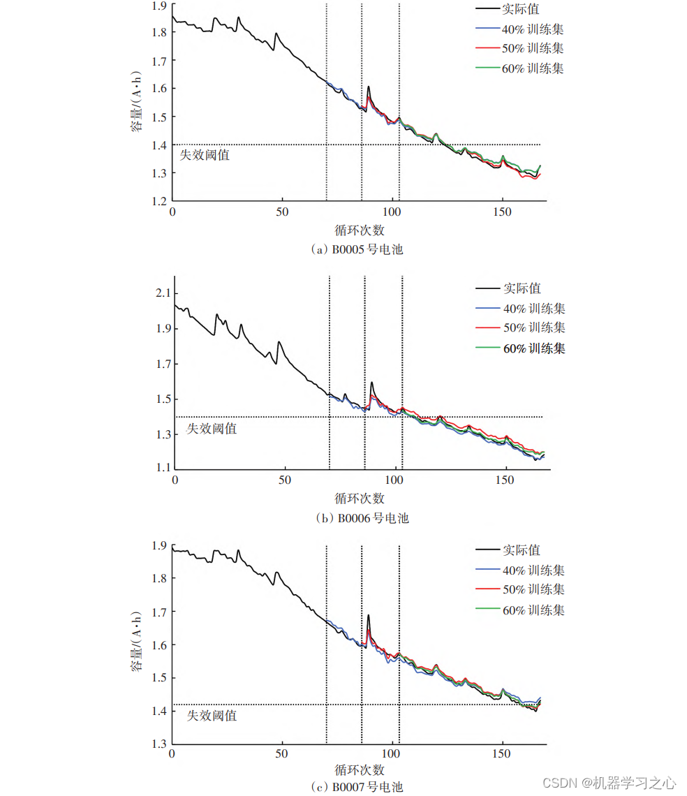
论文辅导 | 基于多尺度分解的LSTM⁃ARIMA锂电池寿命预测
辅导文章 模型描述 锂电池剩余使用寿命(Remaining useful life,RUL)预测是锂电池研究的一个重要方向,通过对RUL的准确预测,可以更好地管理和维护电池,延长电池使用寿命。为了能够准确预测锂电池的RUL&…...

开关阀(4):对于客户技术要求信息的识别
1.阀门部分 2.执行器 行程时间的一般标准 The stroking times are applicable to throttling control valves and should not exceed 2 seconds/inch of valve diameter 3.附件 4.定位器...

Python统计实战:时间序列分析之二阶曲线预测和三阶曲线预测
为了解决特定问题而进行的学习是提高效率的最佳途径。这种方法能够使我们专注于最相关的知识和技能,从而更快地掌握解决问题所需的能力。 (以下练习题来源于《统计学—基于Python》。请在Q群455547227下载原始数据。) 练习题 下表是某只股票…...

Drools开源业务规则引擎(三)- 事件模型(Event Model)
文章目录 Drools开源业务规则引擎(三)- 事件模型(Event Model)1.org.kie.api.event2.RuleRuntimeEventManager3.RuleRuntimeEventListener接口说明示例规则文件规则执行日志输出 4.AgentaEventListener接口说明示例监听器实现类My…...

智慧校园行政办公升级,日程监控不可或缺
在智慧校园的行政办公场景下,日程监控功能扮演了一个核心协调者的角色,它细腻地编织起时间管理的网络,确保各项活动与任务在井然有序中高效推进。这一功能通过以下几个方面,展现了其在提升工作效率与团队协作方面的独特价值。 首先…...

RedHat运维-Linux SSH基础3-sshd守护进程
1. sshd这个守护进程提供了OpenSSH服务,请问可以通过编辑哪些配置文件,来配置这个服务呢?________________________ 2. sshd这个守护进程提供了OpenSSH服务,请问可以通过编辑哪些配置文件,来配置这个服务呢?…...

医院产科信息化管理系统源码,智慧产科管理系统,涵盖了从孕妇到医院初次建档、历次产检、住院分娩、统计上报到产后42天全部医院服务的信息化管理。
医院产科信息化管理系统源码,智慧产科管理系统,产科专科电子病历系统 技术架构:前后端分离Java,Vue,ElementUIMySQL8.0.36 医院产科信息化管理系统,通过构建专科病例系统实现临床保健一体化,涵…...

Softmax作为分类任务中神经网络输出层的优劣分析
Softmax作为分类任务中神经网络输出层的优劣分析 在深度学习领域,Softmax函数作为分类任务中神经网络的输出层,被广泛应用并展现出强大的优势。然而,任何技术都有其两面性,Softmax函数也不例外。本文将从多个角度深入分析Softmax…...

404白色唯美动态页面源码
404白色唯美动态页面源码,源码由HTMLCSSJS组成,记事本打开源码文件可以进行内容文字之类的修改,双击html文件可以本地运行效果,也可以上传到服务器里面,重定向这个界面 404白色唯美动态页面源码...

细说MCU的ADC模块单通道连续采样的实现方法
目录 一、工程依赖的硬件及背景 二、设计目的 三、建立工程 1、配置GPIO 2、选择时钟源和Debug 3、配置ADC 4、配置系统时钟和ADC时钟 5、配置TIM3 6、配置串口 四、代码修改 1、重定义TIM3中断回调函数 2、启动ADC及重写其回调函数 3、定义用于存储转换结果的数…...

H2 Database Console未授权访问漏洞封堵
背景 H2 Database Console未授权访问,默认情况下自动创建不存在的数据库,从而导致未授权访问。各种未授权访问的教程,但是它怎么封堵呢? -ifExists 很简单,启动参数添加 -ifExists ,它的含义:…...

基于java+springboot+vue实现的药店管理系统(文末源码+Lw)285
摘 要 传统信息的管理大部分依赖于管理人员的手工登记与管理,然而,随着近些年信息技术的迅猛发展,让许多比较老套的信息管理模式进行了更新迭代,药品信息因为其管理内容繁杂,管理数量繁多导致手工进行处理不能满足广…...

网络爬虫基础
网络爬虫基础 网络爬虫,也被称为网络蜘蛛或爬虫,是一种用于自动浏览互联网并从网页中提取信息的软件程序。它们能够访问网站,解析页面内容,并收集所需数据。Python语言因其简洁的语法和强大的库支持,成为实现网络爬虫…...

js数组方法归纳——push、pop、unshift、shift
以下涉及到的数组的四个基础方法均会改变原数组!!! 1、 push() 该方法可以向数组的末尾添加一个或多个元素,并返回数组的新的长度可以将要添加的元素作为方法的参数传递,这样这些元素将会自动添加到数组的末尾该方法会将数组新的长度作为返回值返回 //创…...

VPN是什么?
VPN,全称Virtual Private Network,即“虚拟私人网络”,是一种在公共网络(如互联网)上建立加密、安全的连接通道的技术。简单来说,VPN就像是一条在公共道路上铺设的“秘密隧道”,通过这条隧道传输…...

浅析DDoS高防数据中心网络
随着企业业务的持续拓展和数智化转型步伐的加快,数据中心已逐渐演变为企业数据存储、处理和应用的关键部署场地,这也使得数据中心面临着日益严峻的网络安全风险,其中DDoS攻击以其高效性依旧是数据中心面临的主要威胁之一。伴随着数智化的发展…...

《安全行业大模型技术应用态势发展报告(2024)》
人工智能技术快速迭代发展,大模型应用场景不断拓展,随着安全行业对人工智能技术的应用程度日益加深,大模型在网络安全领域的应用潜力和挑战逐渐显现。安全行业大模型技术的应用实践不断涌现,其在威胁检测、风险评估和安全运营等方…...
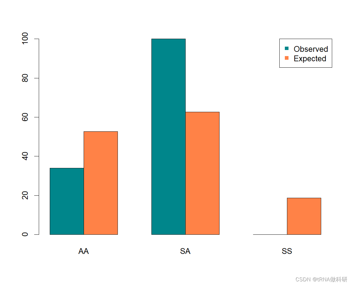
【基于R语言群体遗传学】-4-统计建模与算法(statistical tests and algorithm)
之前的三篇博客,我们对于哈代温伯格遗传比例有了一个全面的认识,没有看的朋友可以先看一下前面的博客: 群体遗传学_tRNA做科研的博客-CSDN博客 1.一些新名词 (1)Algorithm: A series of operations executed in a s…...
结构体的进阶应用)
基于算法竞赛的c++编程(28)结构体的进阶应用
结构体的嵌套与复杂数据组织 在C中,结构体可以嵌套使用,形成更复杂的数据结构。例如,可以通过嵌套结构体描述多层级数据关系: struct Address {string city;string street;int zipCode; };struct Employee {string name;int id;…...
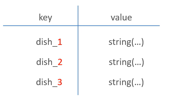
苍穹外卖--缓存菜品
1.问题说明 用户端小程序展示的菜品数据都是通过查询数据库获得,如果用户端访问量比较大,数据库访问压力随之增大 2.实现思路 通过Redis来缓存菜品数据,减少数据库查询操作。 缓存逻辑分析: ①每个分类下的菜品保持一份缓存数据…...

Neo4j 集群管理:原理、技术与最佳实践深度解析
Neo4j 的集群技术是其企业级高可用性、可扩展性和容错能力的核心。通过深入分析官方文档,本文将系统阐述其集群管理的核心原理、关键技术、实用技巧和行业最佳实践。 Neo4j 的 Causal Clustering 架构提供了一个强大而灵活的基石,用于构建高可用、可扩展且一致的图数据库服务…...

数据库分批入库
今天在工作中,遇到一个问题,就是分批查询的时候,由于批次过大导致出现了一些问题,一下是问题描述和解决方案: 示例: // 假设已有数据列表 dataList 和 PreparedStatement pstmt int batchSize 1000; // …...

Pinocchio 库详解及其在足式机器人上的应用
Pinocchio 库详解及其在足式机器人上的应用 Pinocchio (Pinocchio is not only a nose) 是一个开源的 C 库,专门用于快速计算机器人模型的正向运动学、逆向运动学、雅可比矩阵、动力学和动力学导数。它主要关注效率和准确性,并提供了一个通用的框架&…...

JavaScript 数据类型详解
JavaScript 数据类型详解 JavaScript 数据类型分为 原始类型(Primitive) 和 对象类型(Object) 两大类,共 8 种(ES11): 一、原始类型(7种) 1. undefined 定…...

站群服务器的应用场景都有哪些?
站群服务器主要是为了多个网站的托管和管理所设计的,可以通过集中管理和高效资源的分配,来支持多个独立的网站同时运行,让每一个网站都可以分配到独立的IP地址,避免出现IP关联的风险,用户还可以通过控制面板进行管理功…...

DeepSeek源码深度解析 × 华为仓颉语言编程精粹——从MoE架构到全场景开发生态
前言 在人工智能技术飞速发展的今天,深度学习与大模型技术已成为推动行业变革的核心驱动力,而高效、灵活的开发工具与编程语言则为技术创新提供了重要支撑。本书以两大前沿技术领域为核心,系统性地呈现了两部深度技术著作的精华:…...

Python竞赛环境搭建全攻略
Python环境搭建竞赛技术文章大纲 竞赛背景与意义 竞赛的目的与价值Python在竞赛中的应用场景环境搭建对竞赛效率的影响 竞赛环境需求分析 常见竞赛类型(算法、数据分析、机器学习等)不同竞赛对Python版本及库的要求硬件与操作系统的兼容性问题 Pyth…...
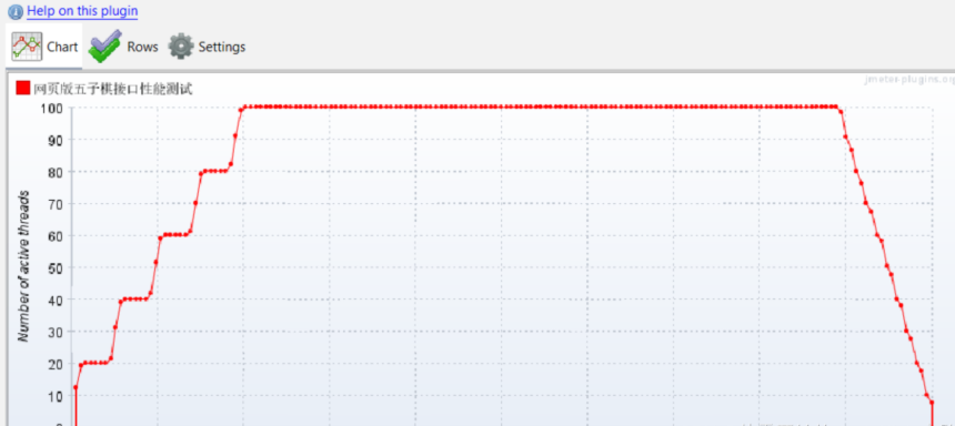
五子棋测试用例
一.项目背景 1.1 项目简介 传统棋类文化的推广 五子棋是一种古老的棋类游戏,有着深厚的文化底蕴。通过将五子棋制作成网页游戏,可以让更多的人了解和接触到这一传统棋类文化。无论是国内还是国外的玩家,都可以通过网页五子棋感受到东方棋类…...