(11)Python引领金融前沿:投资组合优化实战案例
1. 前言
本篇文章为 Python 对金融的投资组合优化的示例。投资组合优化是从一组可用的投资组合中选择最佳投资组合的过程,目的是最大限度地提高回报和降低风险。
投资组合优化是从一组可用的投资组合中选择最佳投资组合的过程,目的是最大限度地提高回报和降低风险。
本案例研究涵盖了我们在前几课中介绍的许多 Python 编程基础知识,例如获取真实世界的市场财务数据、使用 pandas 执行数据分析以及使用 Matplotlib、Seaborn 和 Plotly Express 可视化投资组合数据。
2. 导入库和数据集
在本课中,您将学习如何导入库(例如用于数值分析的 NumPy),并学习如何导入和使用 datetime。此外,您还将学习如何导入数据以执行库提供的一些操作。
在开始之前,我们需要定义以下术语:
-
打开:股票市场开盘时证券首次交易的价格。
-
高:给定股票在常规交易时段内交易的最高价格。
-
低:给定股票在常规交易时段内交易的最低价格。
-
关闭:给定股票在常规交易时段交易的最后价格。
-
卷:开盘和收盘之间的交易股票数量。
-
调整关闭:考虑股票分割和股息后调整后的股票收盘价。
另请注意,纽约证券交易所 (NYSE) 于美国东部时间上午 9:30 开市,上海证券交易所 (SSE) 于中国标准时间上午 9:30 开市。
# Import key librares and modules
import pandas as pd
import numpy as np# Import datetime module that comes pre-installed in Python
# datetime offers classes that work with date & time information
import datetime as dt# Use Pandas to read stock data (the csv file is included in the course package)
stock_df = pd.read_csv('Amazon.csv')
stock_df.head(15)# Count the number of missing values in "stock_df" Pandas DataFrame
stock_df.isnull().sum()# Obtain information about the Pandas DataFrame such as data types, memory utilization..etc
stock_df.info()
3. 计算每日回报率
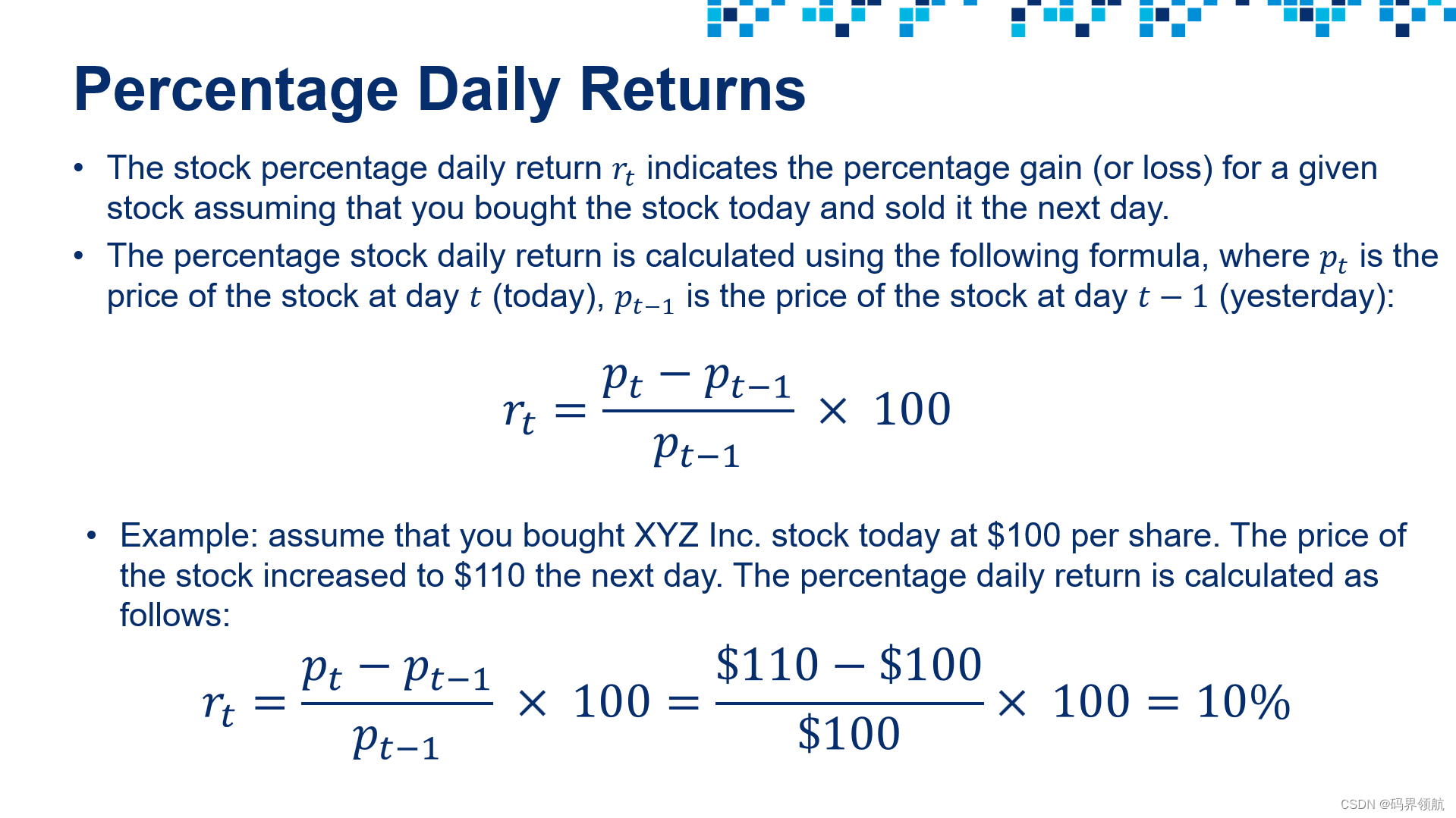
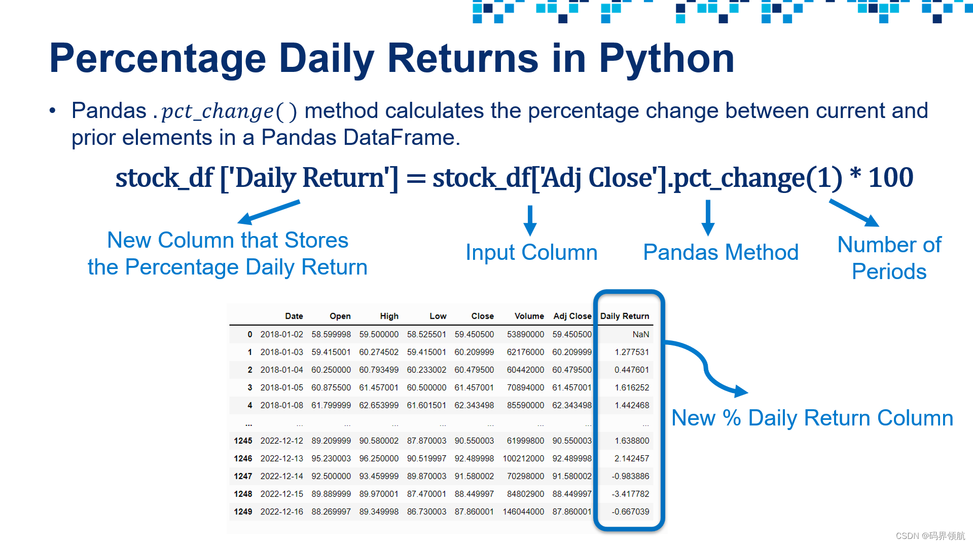
# Calculate the percentage daily return
stock_df['Daily Return'] = stock_df['Adj Close'].pct_change(1) * 100
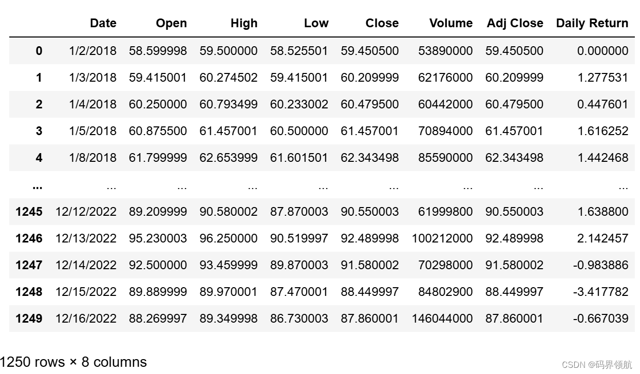
stock_df
输出:

# Let's replace the first row with zeros instead of NaN
stock_df['Daily Return'].replace(np.nan, 0, inplace = True)
stock_df
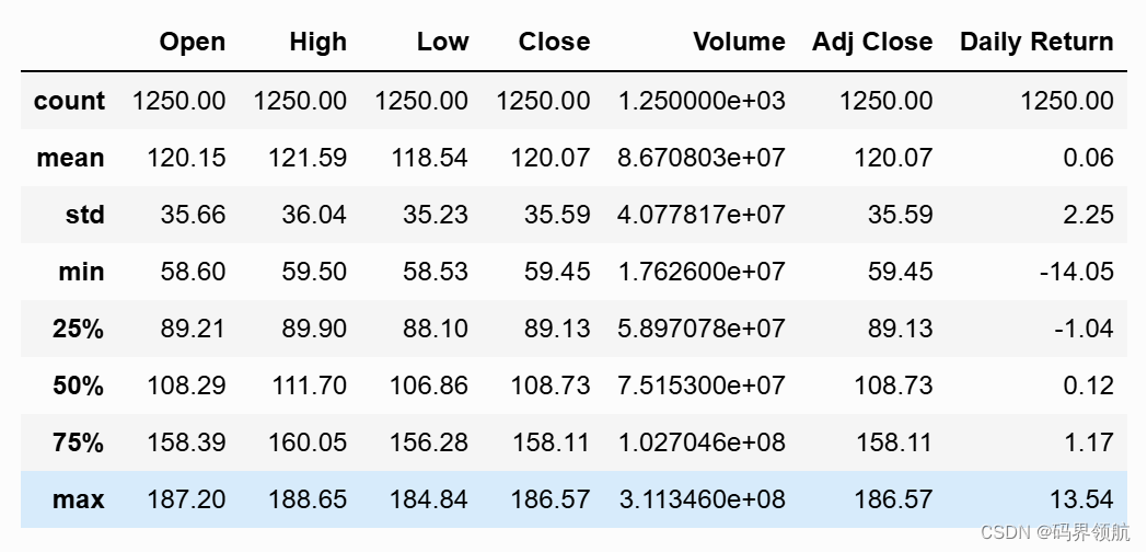
# Use the describe() method to obtain a statistical summary about the data
# Over the specified time period, the average adjusted close price for Amazon stock was $120.07
# The maximum adjusted close price was $186.57
# The maximum volume of shares traded on one day were 311,346,000
stock_df.describe().round(2)
4. 为单只股票进行数据可视化:第一部分
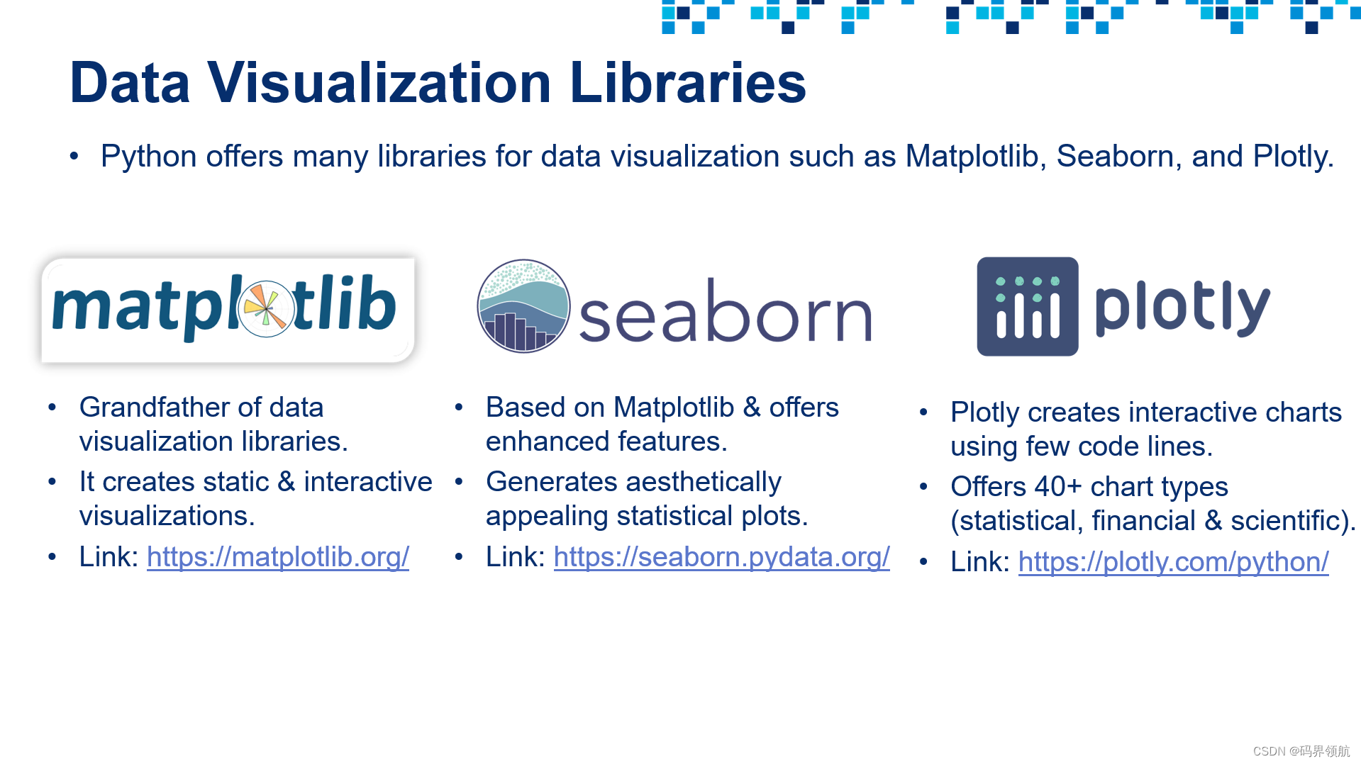
Matplotlib 官方文档: https://matplotlib.org/
Seaborn 官方文档: https://seaborn.pydata.org/
Plotly 官方文档: https://plotly.com/python/
# Matplotlib is a comprehensive data visualization library in Python
# Seaborn is a visualization library that sits on top of matplotlib and offers enhanced features
# plotly.express module contains functions that can create interactive figures using a few lines of codeimport matplotlib.pyplot as plt!pip install seaborn
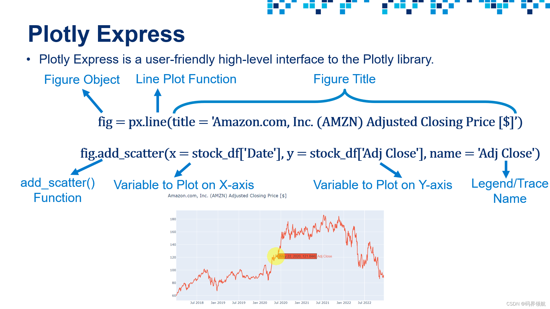
import seaborn as snsimport plotly.express as px# Plot a Line Plot Using Plotly Express
fig = px.line(title = 'Amazon.com, Inc. (AMZN) Adjusted Closing Price [$]')
fig.add_scatter(x = stock_df['Date'], y = stock_df['Adj Close'], name = 'Adj Close')stock_df# Define a function that performs interactive data visualization using Plotly Express
def plot_financial_data(df, title):fig = px.line(title = title)# For loop that plots all stock prices in the pandas dataframe df# Note that index starts with 1 because we want to skip the date columnfor i in df.columns[1:]:fig.add_scatter(x = df['Date'], y = df[i], name = i)fig.update_traces(line_width = 5)fig.update_layout({'plot_bgcolor': "white"})fig.show()# Plot High, Low, Open, Close and Adj Close
plot_financial_data(stock_df.drop(['Volume', 'Daily Return'], axis = 1), 'Amazon.com, Inc. (AMZN) Stock Price [$]')# Plot trading volume
plot_financial_data(stock_df.iloc[:,[0,5]], 'Amazon.com, Inc. (AMZN) Trading Volume')# Plot % Daily Returns
plot_financial_data(stock_df.iloc[:,[0,7]], 'Amazon.com, Inc. (AMZN) Percentage Daily Return [%]')
5. 为单只股票进行数据可视化:第二部分
# Define a function that classifies the returns based on the magnitude
# Feel free to change these numbers
def percentage_return_classifier(percentage_return):if percentage_return > -0.3 and percentage_return <= 0.3:return 'Insignificant Change'elif percentage_return > 0.3 and percentage_return <= 3:return 'Positive Change'elif percentage_return > -3 and percentage_return <= -0.3:return 'Negative Change'elif percentage_return > 3 and percentage_return <= 7:return 'Large Positive Change'elif percentage_return > -7 and percentage_return <= -3:return 'Large Negative Change'elif percentage_return > 7:return 'Bull Run'elif percentage_return <= -7:return 'Bear Sell Off'# Apply the function to the "Daily Return" Column and place the result in "Trend" column
stock_df['Trend'] = stock_df['Daily Return'].apply(percentage_return_classifier)
stock_df# Count distinct values in the Trend column
trend_summary = stock_df['Trend'].value_counts()
trend_summary# Plot a pie chart using Matplotlib Library
plt.figure(figsize = (8, 8))
trend_summary.plot(kind = 'pie', y = 'Trend');# Plot a pie chart using Matplotlib Library
plt.figure(figsize = (8, 8))
trend_summary.plot(kind = 'pie', y = 'Trend');
6. 为单只股票进行数据可视化:第三部分
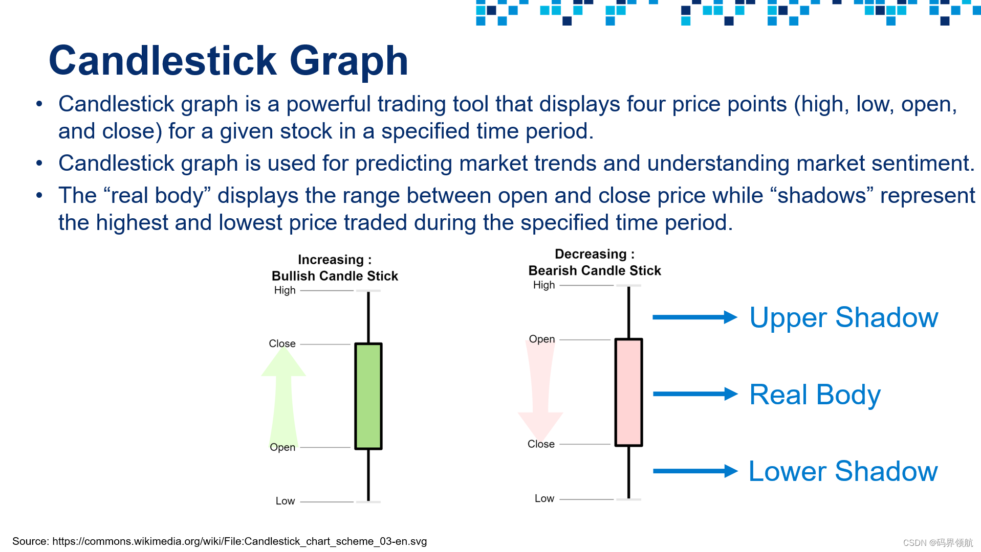
# Let's plot a candlestick graph using Cufflinks library
# Cufflinks is a powerful Python library that connects Pandas and Plotly for generating plots using few lines of code
# Cufflinks allows for interactive data visualization
! pip install cufflinks
import cufflinks as cf
cf.go_offline() # Enabling offline mode for interactive data visualization locallystock_df# Set the date to be the index for the Pandas DataFrame
# This is critical to show the date on the x-axis when using cufflinks
stock_df.set_index(['Date'], inplace = True)
stock_df# Plot Candlestick figure using Cufflinks QuantFig module
figure = cf.QuantFig(stock_df, title = 'Amazon.com, Inc. (AMZN) Candlestick Chart', name = 'AMZN')
figure.add_sma(periods =[14, 21], column = 'Close', color = ['magenta', 'green'])
figure.iplot(theme = 'white', up_color = 'green', down_color = 'red')
7. 为多只股票进行数据可视化
# Let's read multiple stocks data contained in "stock_prices.csv" attached in the course package
# The Appendix includes details on how to obtain this data using yfinance and Pandas Datareader
# Note that yfinance and Pandas Datareader might experience outage in some geographical regions# We will focus our analysis on U.S. stocks, similar analysis could be performed on Asian, European or African stocks
# AMZN: Amazon Inc. - Multinational tech company focusing on e-commerce, cloud computing, and artificial intelligence
# JPM: JPMorgan Chase and Co. - Multinational investment bank and financial services holding company
# META: Meta Platforms, formerly named Facebook Inc. - META owns Facebook, Instagram, and WhatsApp
# PG: Procter and Gamble (P&G) - Multinational consumer goods corporation
# GOOG: Google (Alphabet Inc.) - Multinational company that focuses on search engine tech, e-commerce, Cloud and AI
# CAT: Caterpillar - World's largest construction-equipment manufacturer
# PFE: Pfizer Inc. - Multinational pharmaceutical and biotechnology corporation
# EXC: Exelon - An American Fortune 100 energy company
# DE: Deere & Company (John Deere) - Manufactures agricultural machinery and heavy equipment
# JNJ: Johnson & Johnson - A multinational corporation that develops medical devices and pharmaceuticalsclose_price_df = pd.read_csv('stock_prices.csv')
close_price_df# The objective of this code cell is to calculate the percentage daily return
# We will perform this calculation on all stocks except for the first column which is "Date"
daily_returns_df = close_price_df.iloc[:, 1:].pct_change() * 100
daily_returns_df.replace(np.nan, 0, inplace = True)
daily_returns_df# Insert the date column at the start of the Pandas DataFrame (@ index = 0)
daily_returns_df.insert(0, "Date", close_price_df['Date'])
daily_returns_df# Plot closing prices using plotly Express. Note that we used the same pre-defined function "plot_financial_data"
plot_financial_data(close_price_df, 'Adjusted Closing Prices [$]')# Plot the stocks daily returns
plot_financial_data(daily_returns_df, 'Percentage Daily Returns [%]')# Plot histograms for stocks daily returns using plotly express
# Compare META to JNJ daily returns histograms
fig = px.histogram(daily_returns_df.drop(columns = ['Date']))
fig.update_layout({'plot_bgcolor': "white"})# Plot a heatmap showing the correlations between daily returns
# Strong positive correlations between Catterpillar and John Deere - both into heavy equipment and machinery
# META and Google - both into Tech and Cloud Computing
plt.figure(figsize = (10, 8))
sns.heatmap(daily_returns_df.drop(columns = ['Date']).corr(), annot = True);# Plot the Pairplot between stocks daily returns
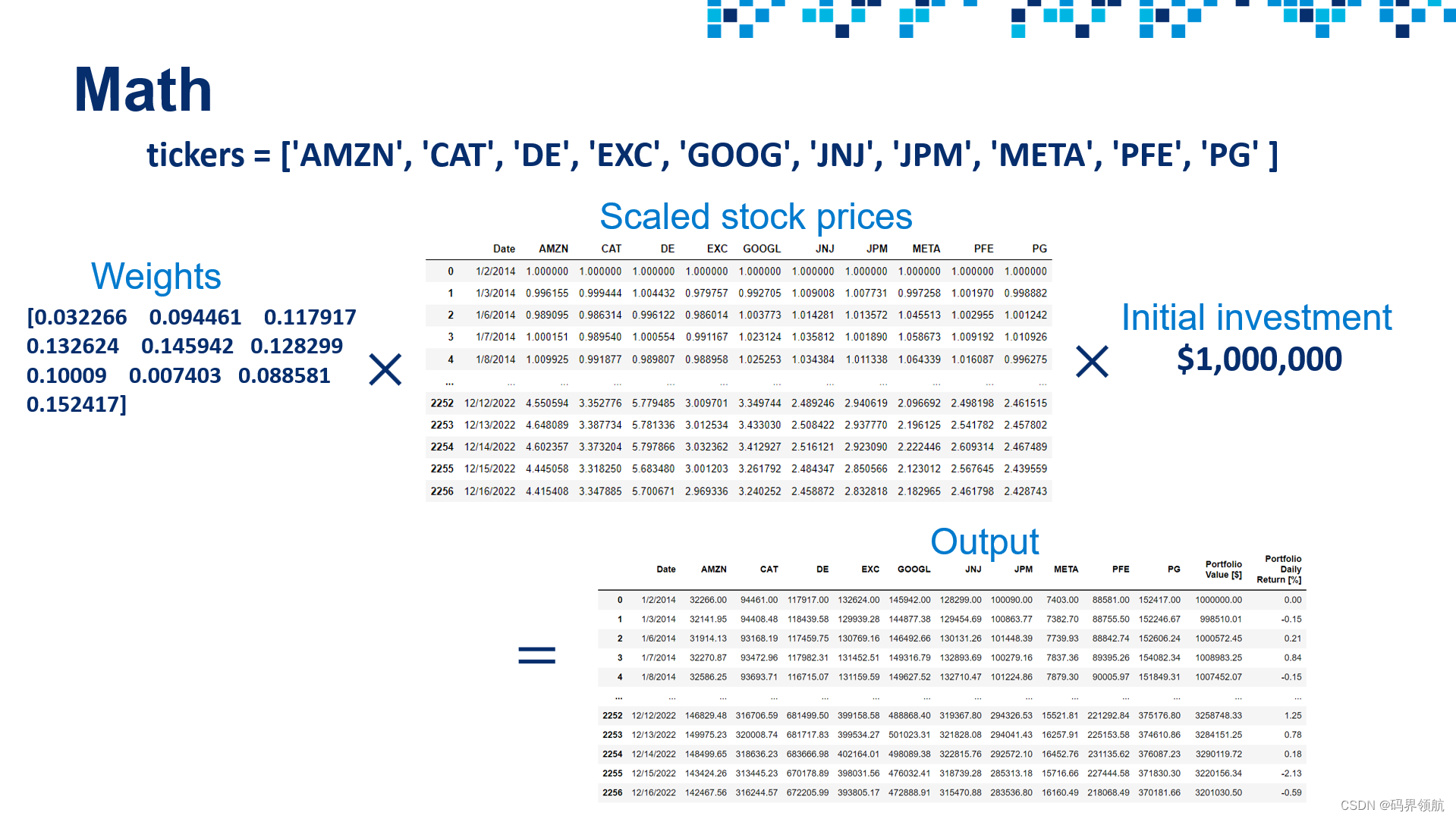
sns.pairplot(daily_returns_df);# Function to scale stock prices based on their initial starting price
# The objective of this function is to set all prices to start at a value of 1
def price_scaling(raw_prices_df):scaled_prices_df = raw_prices_df.copy()for i in raw_prices_df.columns[1:]:scaled_prices_df[i] = raw_prices_df[i]/raw_prices_df[i][0]return scaled_prices_dfprice_scaling(close_price_df)
8. 定义一个生成随机投资组合权重的函数
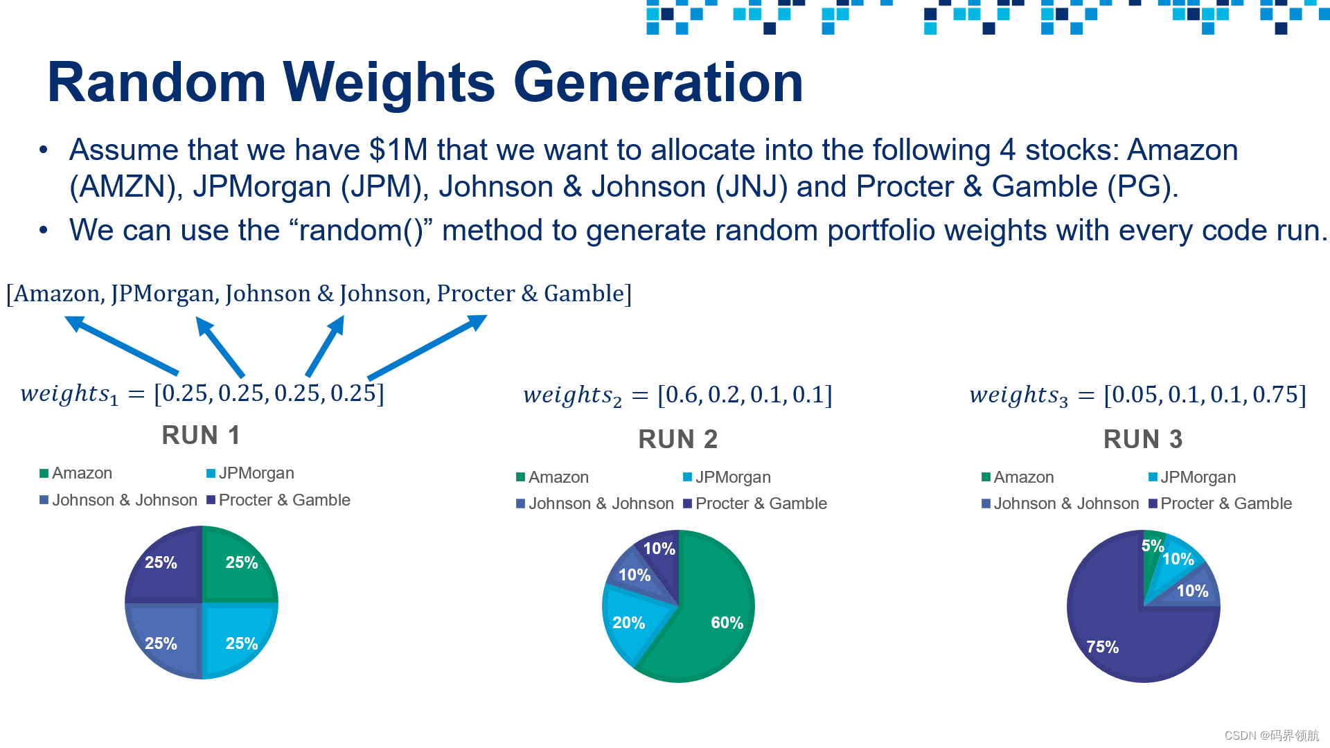
# Let's create an array that holds random portfolio weights
# Note that portfolio weights must add up to 1
import randomdef generate_portfolio_weights(n):weights = []for i in range(n):weights.append(random.random())# let's make the sum of all weights add up to 1weights = weights/np.sum(weights)return weights# Call the function (Run this cell multiple times to generate different outputs)
weights = generate_portfolio_weights(4)
print(weights)
9. 进行资产配置并计算投资组合的日价值/回报率
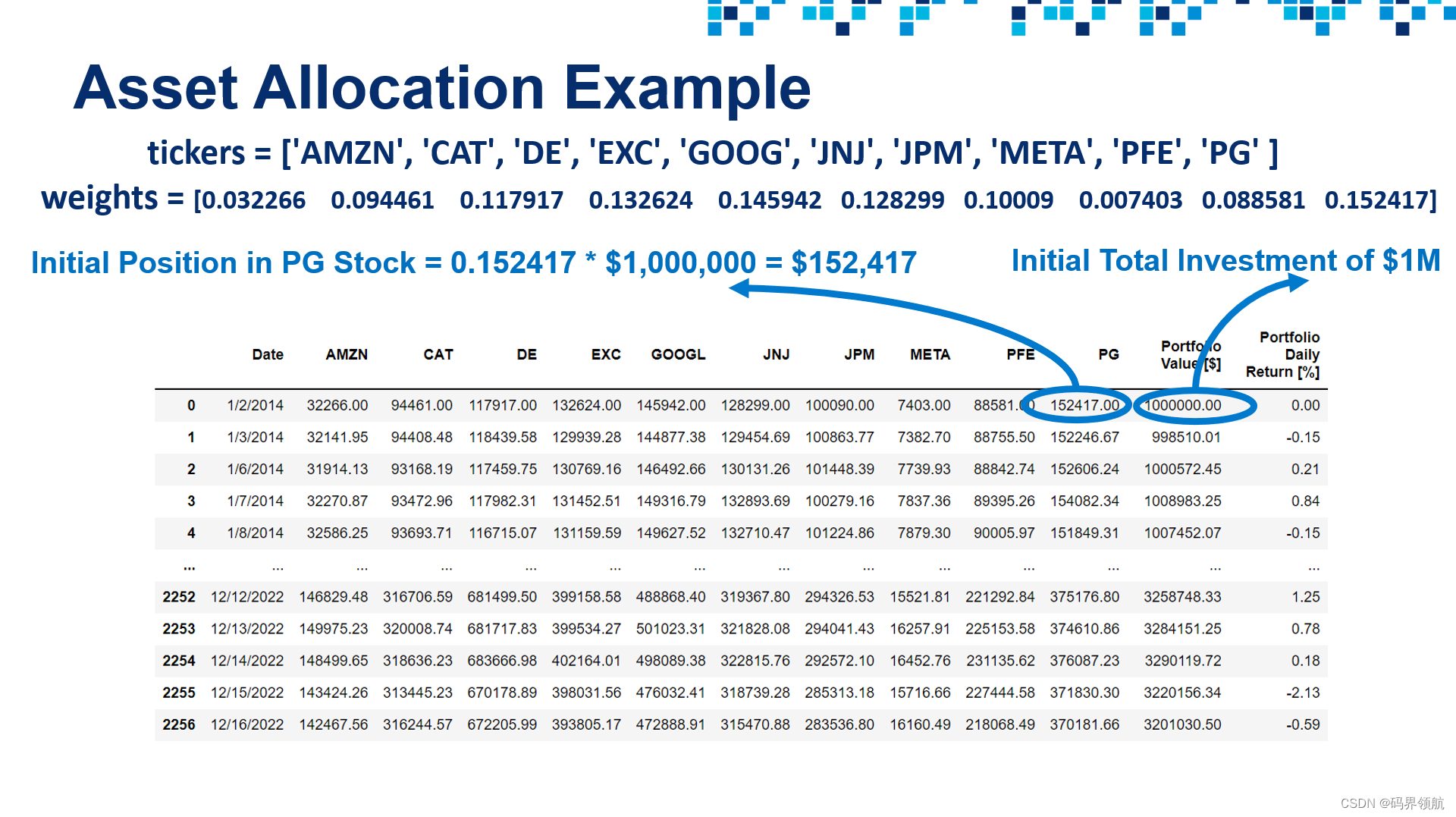

# Let's define the "weights" list similar to the slides
weights = [0.032266, 0.094461, 0.117917, 0.132624, 0.145942, 0.128299, 0.10009, 0.007403, 0.088581, 0.152417]
weights# Let's display "close_price_df" Pandas DataFrame
close_price_df# Scale stock prices using the "price_scaling" function that we defined earlier (make all stock values start at 1)
portfolio_df = close_price_df.copy()
scaled_df = price_scaling(portfolio_df)
scaled_df# Use enumerate() method to obtain the stock names along with a counter "i" (0, 1, 2, 3,..etc.)
# This counter "i" will be used as an index to access elements in the "weights" list
initial_investment = 1000000
for i, stock in enumerate(scaled_df.columns[1:]):portfolio_df[stock] = weights[i] * scaled_df[stock]  * initial_investment
portfolio_df.round(1)# Assume that we have $1,000,000 that we would like to invest in one or more of the selected stocks
# Let's create a function that receives the following arguments: # (1) Stocks closing prices# (2) Random weights # (3) Initial investment amount
# The function will return a DataFrame that contains the following:# (1) Daily value (position) of each individual stock over the specified time period# (2) Total daily value of the portfolio # (3) Percentage daily return def asset_allocation(df, weights, initial_investment):portfolio_df = df.copy()# Scale stock prices using the "price_scaling" function that we defined earlier (Make them all start at 1)scaled_df = price_scaling(df)for i, stock in enumerate(scaled_df.columns[1:]):portfolio_df[stock] = scaled_df[stock] * weights[i] * initial_investment# Sum up all values and place the result in a new column titled "portfolio value [$]" # Note that we excluded the date column from this calculationportfolio_df['Portfolio Value [$]'] = portfolio_df[portfolio_df != 'Date'].sum(axis = 1, numeric_only = True)# Calculate the portfolio percentage daily return and replace NaNs with zerosportfolio_df['Portfolio Daily Return [%]'] = portfolio_df['Portfolio Value [$]'].pct_change(1) * 100 portfolio_df.replace(np.nan, 0, inplace = True)return portfolio_df# Now let's put this code in a function and generate random weights
# Let's obtain the number of stocks under consideration (note that we ignored the "Date" column)
n = len(close_price_df.columns)-1# Let's generate random weights
print('Number of stocks under consideration = {}'.format(n))
weights = generate_portfolio_weights(n).round(6)
print('Portfolio weights = {}'.format(weights))# Let's test out the "asset_allocation" function
portfolio_df = asset_allocation(close_price_df, weights, 1000000)
portfolio_df.round(2)# Plot the portfolio percentage daily return
plot_financial_data(portfolio_df[['Date', 'Portfolio Daily Return [%]']], 'Portfolio Percentage Daily Return [%]')# Plot each stock position in our portfolio over time
# This graph shows how our initial investment in each individual stock grows over time
plot_financial_data(portfolio_df.drop(['Portfolio Value [$]', 'Portfolio Daily Return [%]'], axis = 1), 'Portfolio positions [$]')# Plot the total daily value of the portfolio (sum of all positions)
plot_financial_data(portfolio_df[['Date', 'Portfolio Value [$]']], 'Total Portfolio Value [$]')
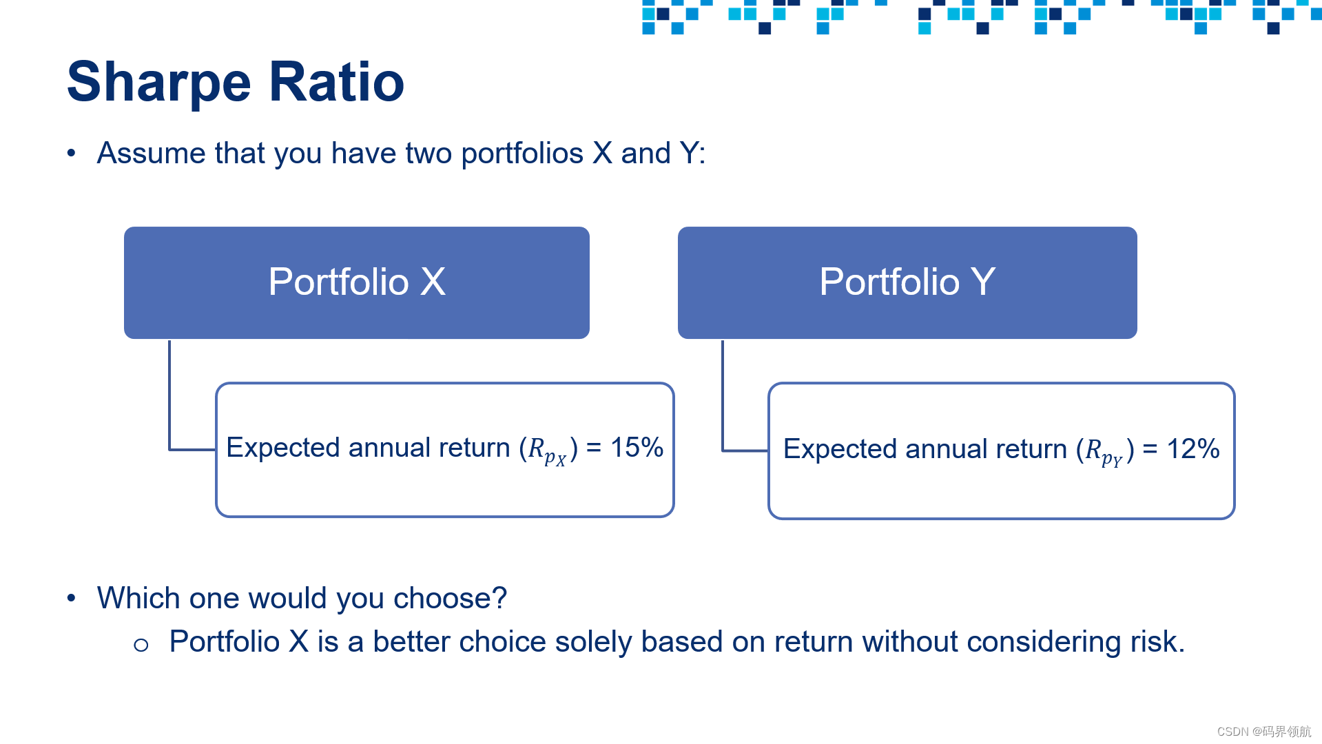
10. 定义“模拟”函数,该函数执行资产配置并计算关键的投资组合指标

# Let's define the simulation engine function
# The function receives: # (1) portfolio weights# (2) initial investment amount
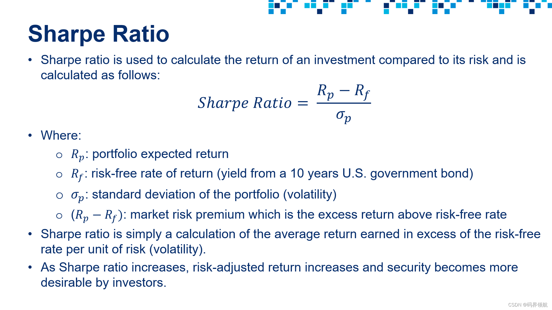
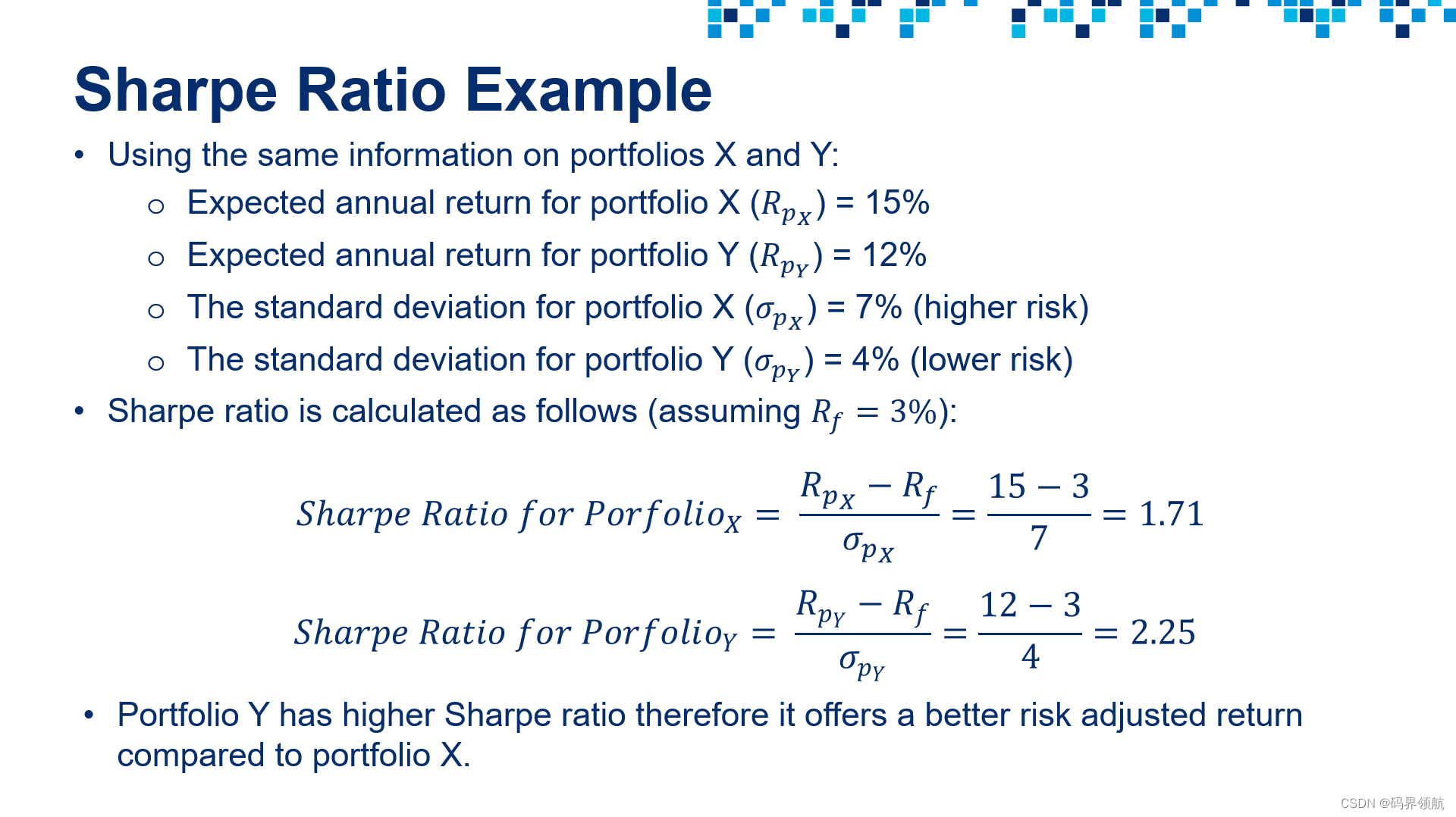
# The function performs asset allocation and calculates portfolio statistical metrics including Sharpe ratio
# The function returns: # (1) Expected portfolio return # (2) Expected volatility # (3) Sharpe ratio # (4) Return on investment # (5) Final portfolio value in dollarsdef simulation_engine(weights, initial_investment):# Perform asset allocation using the random weights (sent as arguments to the function)portfolio_df = asset_allocation(close_price_df, weights, initial_investment)# Calculate the return on the investment # Return on investment is calculated using the last final value of the portfolio compared to its initial valuereturn_on_investment = ((portfolio_df['Portfolio Value [$]'][-1:] - portfolio_df['Portfolio Value [$]'][0])/ portfolio_df['Portfolio Value [$]'][0]) * 100# Daily change of every stock in the portfolio (Note that we dropped the date, portfolio daily worth and daily % returns) portfolio_daily_return_df = portfolio_df.drop(columns = ['Date', 'Portfolio Value [$]', 'Portfolio Daily Return [%]'])portfolio_daily_return_df = portfolio_daily_return_df.pct_change(1) # Portfolio Expected Return formulaexpected_portfolio_return = np.sum(weights * portfolio_daily_return_df.mean() ) * 252# Portfolio volatility (risk) formula# The risk of an asset is measured using the standard deviation which indicates the dispertion away from the mean# The risk of a portfolio is not a simple sum of the risks of the individual assets within the portfolio# Portfolio risk must consider correlations between assets within the portfolio which is indicated by the covariance # The covariance determines the relationship between the movements of two random variables# When two stocks move together, they have a positive covariance when they move inversely, the have a negative covariance covariance = portfolio_daily_return_df.cov() * 252 expected_volatility = np.sqrt(np.dot(weights.T, np.dot(covariance, weights)))# Check out the chart for the 10-years U.S. treasury at https://ycharts.com/indicators/10_year_treasury_raterf = 0.03 # Try to set the risk free rate of return to 1% (assumption)# Calculate Sharpe ratiosharpe_ratio = (expected_portfolio_return - rf)/expected_volatility return expected_portfolio_return, expected_volatility, sharpe_ratio, portfolio_df['Portfolio Value [$]'][-1:].values[0], return_on_investment.values[0]# Let's test out the "simulation_engine" function and print out statistical metrics
# Define the initial investment amount
initial_investment = 1000000
portfolio_metrics = simulation_engine(weights, initial_investment)print('Expected Portfolio Annual Return = {:.2f}%'.format(portfolio_metrics[0] * 100))
print('Portfolio Standard Deviation (Volatility) = {:.2f}%'.format(portfolio_metrics[1] * 100))
print('Sharpe Ratio = {:.2f}'.format(portfolio_metrics[2]))
print('Portfolio Final Value = ${:.2f}'.format(portfolio_metrics[3]))
print('Return on Investment = {:.2f}%'.format(portfolio_metrics[4]))11. 运行蒙特卡罗模拟

# Set the number of simulation runs
sim_runs = 10000
initial_investment = 1000000# Placeholder to store all weights
weights_runs = np.zeros((sim_runs, n))# Placeholder to store all Sharpe ratios
sharpe_ratio_runs = np.zeros(sim_runs)# Placeholder to store all expected returns
expected_portfolio_returns_runs = np.zeros(sim_runs)# Placeholder to store all volatility values
volatility_runs = np.zeros(sim_runs)# Placeholder to store all returns on investment
return_on_investment_runs = np.zeros(sim_runs)# Placeholder to store all final portfolio values
final_value_runs = np.zeros(sim_runs)for i in range(sim_runs):# Generate random weights weights = generate_portfolio_weights(n)# Store the weightsweights_runs[i,:] = weights# Call "simulation_engine" function and store Sharpe ratio, return and volatility# Note that asset allocation is performed using the "asset_allocation" function  expected_portfolio_returns_runs[i], volatility_runs[i], sharpe_ratio_runs[i], final_value_runs[i], return_on_investment_runs[i] = simulation_engine(weights, initial_investment)print("Simulation Run = {}".format(i))   print("Weights = {}, Final Value = ${:.2f}, Sharpe Ratio = {:.2f}".format(weights_runs[i].round(3), final_value_runs[i], sharpe_ratio_runs[i]))   print('\n')
12. 执行投资组合优化
# List all Sharpe ratios generated from the simulation
sharpe_ratio_runs# Return the index of the maximum Sharpe ratio (Best simulation run)
sharpe_ratio_runs.argmax()# Return the maximum Sharpe ratio value
sharpe_ratio_runs.max()weights_runs# Obtain the portfolio weights that correspond to the maximum Sharpe ratio (Golden set of weights!)
weights_runs[sharpe_ratio_runs.argmax(), :]# Return Sharpe ratio, volatility corresponding to the best weights allocation (maximum Sharpe ratio)
optimal_portfolio_return, optimal_volatility, optimal_sharpe_ratio, highest_final_value, optimal_return_on_investment = simulation_engine(weights_runs[sharpe_ratio_runs.argmax(), :], initial_investment)print('Best Portfolio Metrics Based on {} Monte Carlo Simulation Runs:'.format(sim_runs))
print(' - Portfolio Expected Annual Return = {:.02f}%'.format(optimal_portfolio_return * 100))
print(' - Portfolio Standard Deviation (Volatility) = {:.02f}%'.format(optimal_volatility * 100))
print(' - Sharpe Ratio = {:.02f}'.format(optimal_sharpe_ratio))
print(' - Final Value = ${:.02f}'.format(highest_final_value))
print(' - Return on Investment = {:.02f}%'.format(optimal_return_on_investment))# Create a DataFrame that contains volatility, return, and Sharpe ratio for all simualation runs
sim_out_df = pd.DataFrame({'Volatility': volatility_runs.tolist(), 'Portfolio_Return': expected_portfolio_returns_runs.tolist(), 'Sharpe_Ratio': sharpe_ratio_runs.tolist() })
sim_out_df# Plot volatility vs. return for all simulation runs
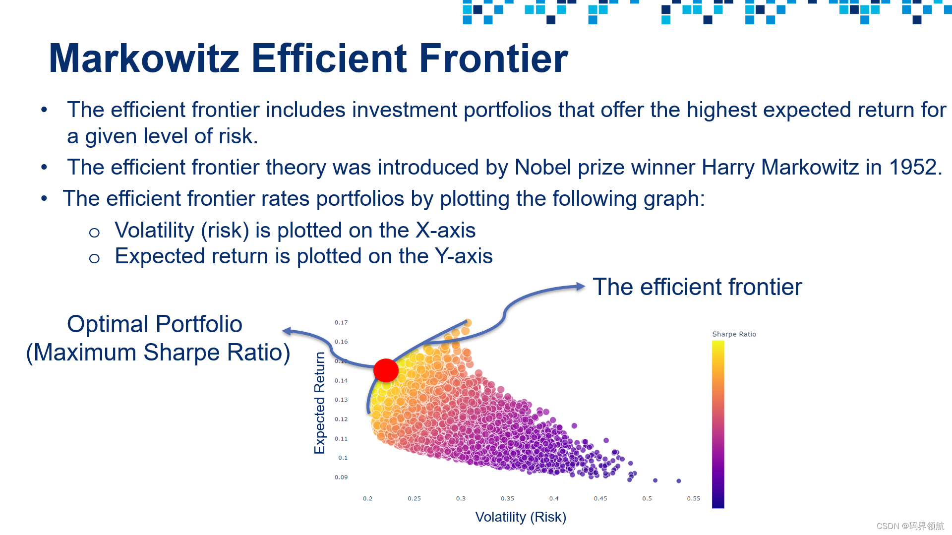
# Highlight the volatility and return that corresponds to the highest Sharpe ratio
import plotly.graph_objects as go
fig = px.scatter(sim_out_df, x = 'Volatility', y = 'Portfolio_Return', color = 'Sharpe_Ratio', size = 'Sharpe_Ratio', hover_data = ['Sharpe_Ratio'] )
fig.update_layout({'plot_bgcolor': "white"})
fig.show()# Use this code if Sharpe ratio is negative
# fig = px.scatter(sim_out_df, x = 'Volatility', y = 'Portfolio_Return', color = 'Sharpe_Ratio', hover_data = ['Sharpe_Ratio'] )# Let's highlight the point with the highest Sharpe ratio
fig = px.scatter(sim_out_df, x = 'Volatility', y = 'Portfolio_Return', color = 'Sharpe_Ratio', size = 'Sharpe_Ratio', hover_data = ['Sharpe_Ratio'] )
fig.add_trace(go.Scatter(x = [optimal_volatility], y = [optimal_portfolio_return], mode = 'markers', name = 'Optimal Point', marker = dict(size=[40], color = 'red')))
fig.update_layout(coloraxis_colorbar = dict(y = 0.7, dtick = 5))
fig.update_layout({'plot_bgcolor': "white"})
fig.show()
相关文章:
(11)Python引领金融前沿:投资组合优化实战案例
1. 前言 本篇文章为 Python 对金融的投资组合优化的示例。投资组合优化是从一组可用的投资组合中选择最佳投资组合的过程,目的是最大限度地提高回报和降低风险。 投资组合优化是从一组可用的投资组合中选择最佳投资组合的过程,目的是最大限度地提高回报…...

git删除本地远程分支
gitlab删除远程分支 要删除GitLab上的远程分支,你可以使用Git命令行工具。以下是删除远程分支的步骤和示例代码: 首先,确保你已经在本地删除了分支。删除本地分支的命令是: git branch -d <branch_name> 如果分支没有被合…...
前端-04-VScode敲击键盘有键入音效,怎么关闭
目录 问题解决办法 问题 今天正在VScode敲项目,不知道是按了什么快捷键还是什么的,敲击键盘有声音,超级烦人啊!!于是我上网查了一下,应该是开启了VScode的键入音效,下面是关闭键入音效的办法。…...

JMeter数据库连接操作及断言
一、数据库操作 应用场景: 接口自动化数据校验:用于验证接口返回的数据与数据库中的数据是否一致。特殊业务:处理一些与数据库相关的特殊业务逻辑。性能测试:测试数据库的性能,如查询、更新等操作的响应时间。 连接数…...

Maven settings.xml 私服上传和拉取配置
公司内部自行开发的依赖包需要上传到maven私服时,可以在项目的pom.xml中配置,也可以在本地计算机的maven目录settings.xml中配置。本文讲述的是如何在settings.xml中进行配置。 场景:有两个maven私服,其中一个为公司的࿰…...

【STM32】MPU内存保护单元
注:仅在F7和M7系列上使用介绍 功能: 设置不同存储区域的存储器访问权限(管理员、用户) 设置存储器(内存和外设)属性(可缓冲、可缓存、可共享) 优点:提高嵌入式系统的健壮…...

用Python爬虫能实现什么?
Python 是进行网络爬虫开发的一个非常流行和强大的语言,这主要得益于其丰富的库和框架,比如 requests、BeautifulSoup、Scrapy 等。下面我将简要介绍 Python 爬虫的基础知识和几个关键步骤。 1. 爬虫的基本原理 网络爬虫(Web Crawler&#…...

【QT】label中添加QImage图片并旋转(水平翻转、垂直翻转、顺时针旋转、逆时针旋转)
目录 0.简介 1.详细代码及解释 1)原label显示在界面上 2)水平翻转 3)垂直翻转 4)顺时针旋转45度 5)逆时针旋转 0.简介 环境:windows11 QtCreator 背景:demo,父类为QWidget&a…...

CSP-J模拟赛day1
yjq的吉祥数 文件读写 输入文件 a v o i d . i n avoid.in avoid.in 输出文件 a v o i d . o u t avoid.out avoid.out 限制 1000ms 512MB 题目描述 众所周知, 这个数字在有些时候不是很吉利,因为它谐音为 “散” 所以yjq认为只要是 的整数次幂的数…...
Docker构建LNMP环境并运行Wordpress平台
1.准备Nginx 上传文件 Dockerfile FROM centos:7 as firstADD nginx-1.24.0.tar.gz /opt/ COPY CentOS-Base.repo /etc/yum.repos.d/RUN yum -y install pcre-devel zlib-devel openssl-devel gcc gcc-c make && \useradd -M -s /sbin/nologin nginx && \cd /o…...

《峡谷小狐仙-多模态角色扮演游戏助手》复现流程
YongXie66/Honor-of-Kings_RolePlay: The Role Playing Project of Honor-of-Kings Based on LnternLM2。峡谷小狐仙--王者荣耀领域的角色扮演聊天机器人,结合多模态技术将英雄妲己的形象带入大模型中。 (github.com) https://github.com/chg0901/Honor_of_Kings…...
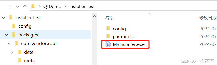
Qt 使用Installer Framework制作安装包
Qt 使用Installer Framework制作安装包 引言一、下载安装 Qt Installer Framework二、简单使用2.1 创建目录结构 (文件夹结构)2.2 制作程序压缩包2.3 制作程序安装包 引言 Qt Installer Framework (安装程序框架)是一个强大的工具集,用于创建自定义的在线和离线安装…...

Typora 1.5.8 版本安装下载教程 (轻量级 Markdown 编辑器),图文步骤详解,免费领取(软件可激活使用)
文章目录 软件介绍软件下载安装步骤激活步骤 软件介绍 Typora是一款基于Markdown语法的轻量级文本编辑器,它的主要目标是为用户提供一个简洁、高效的写作环境。以下是Typora的一些主要特点和功能: 实时预览:Typora支持实时预览功能࿰…...

linux代填密码切换用户
一、背景 linux用户账户密码复杂,在不考虑安全的情况下,想要使用命令自动切换用户 二、操作 通过 expect 工具来实现自动输入密码的效果 yum install expect创建switchRoot.exp文件,内容参考下面的 #!/usr/bin/expect set username root…...

防火墙的经典体系结构及其具体结构
防火墙的经典体系结构及其具体结构 防火墙是保护计算机网络安全的重要设备或软件,主要用于监控和控制进出网络流量,防止未经授权的访问。防火墙的经典体系结构主要包括包过滤防火墙、状态检测防火墙、代理防火墙和下一代防火墙(NGFW…...
【BUG】已解决:note: This is an issue with the package mentioned above,not pip.
已解决:note: This is an issue with the package mentioned above,not pip. 欢迎来到英杰社区https://bbs.csdn.net/topics/617804998 欢迎来到我的主页,我是博主英杰,211科班出身,就职于医疗科技公司,热衷…...
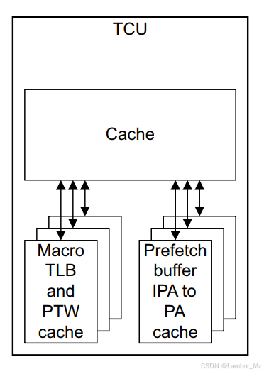
【ARM】SMMU系统虚拟化整理
目录 1.MMU的基本介绍 1.1 特点梳理 2.功能 DVM interface PTW interface 2.1 操作流程 2.1.1 StreamID 2.1.2 安全状态: 2.1.3 HUM 2.1.4 可配置的操作特性 Outstanding transactions per TBU QoS 仲裁 2.2 Cache结构 2.2.1 Micro TLB 2.2.2 Macro…...

PYQT按键长按机制
长按按键不松开也会触发 keyReleaseEvent 事件,是由于操作系统的键盘事件处理机制。大多数操作系统在检测到键盘按键被长按时,会重复生成按键按下 (keyPressEvent) 和按键释放 (keyReleaseEvent) 事件。这种行为通常被称为“键盘自动重复”。 通过检测 …...
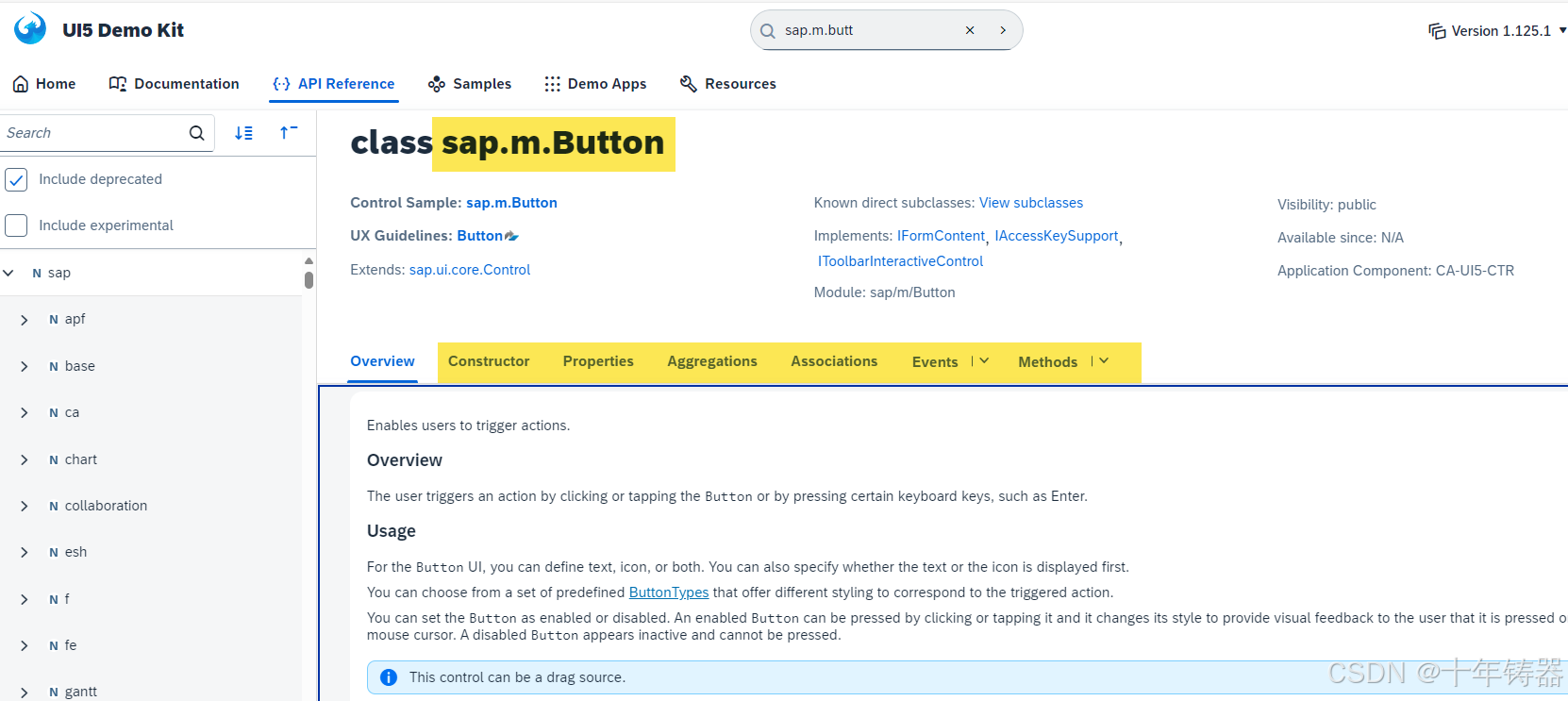
SAPUI5基础知识15 - 理解控件的本质
1. 背景 经过一系列的练习,通过不同的SAPUI5控件,我们完成了对应用程序界面的初步设计,在本篇博客中,让我们一起总结下SAPUI5控件的相关知识点,更深入地理解SAPUI5控件的本质。 通常而言,一个典型UI5应用…...

十七、【机器学习】【非监督学习】- K-均值 (K-Means)
系列文章目录 第一章 【机器学习】初识机器学习 第二章 【机器学习】【监督学习】- 逻辑回归算法 (Logistic Regression) 第三章 【机器学习】【监督学习】- 支持向量机 (SVM) 第四章【机器学习】【监督学习】- K-近邻算法 (K-NN) 第五章【机器学习】【监督学习】- 决策树…...

Visual StudioProfiler对工作流进行热点分析
热点:消耗了绝大部分CPU计算时间(例如超过50%或更高比例)的那部分代码。Visual Studio 中,使用性能探查器(Profiler)在 Visual Studio 中,使用性能探查器(Profiler)进行热…...

百度文库免vip下载文档_百度文库vip兑换码
这个还是我朋友给我说的一个工具,可以直接下载文档。也不需要登录会员。给大家看一下。方法在这:点我去下载 这个就是测试下载的文档,还是不错的。大家有需要可以去试试看 今日密码在这...

C/C++: 栈包含哪些数据信息
函数参数 (32、64位的参数传递又不一样,ABI) 局部变量; 临时寄存器保存; 栈地址指针,栈底寄存器; 指令返回地址; The frame is the area on the stack that holds local variables and saved registers 所以导致栈溢出的情况,一般就是局部变量,这个可注入的点。函数参…...

MiniGrid 开源项目教程
MiniGrid 开源项目教程 【免费下载链接】minigrid 📏 Minimal 2kb zero dependency cascading grid layout 项目地址: https://gitcode.com/gh_mirrors/min/minigrid 1. 项目的目录结构及介绍 MiniGrid 项目的目录结构如下: minigrid/ ├── R…...

开源项目 Adobe-GenP 的扩展与二次开发潜力
开源项目 Adobe-GenP 的扩展与二次开发潜力 【免费下载链接】Adobe-GenP Adobe CC 2019/2020/2021/2022/2023 GenP Universal Patch 3.0 项目地址: https://gitcode.com/gh_mirrors/ad/Adobe-GenP 1. 项目的基础介绍 Adobe-GenP 是一个开源项目,旨在提供一种…...

Android Studio项目难题解决:Qwen3-14B-Int4-AWQ调试Gradle构建错误与UI设计
Android Studio项目难题解决:Qwen3-14B-Int4-AWQ调试Gradle构建错误与UI设计 1. 引言:当Android开发遇上AI助手 作为一名Android开发者,你是否经历过这样的场景:深夜赶项目时Gradle突然报错,红色错误日志铺满屏幕&am…...

NEURAL MASK 数据库集成实战:管理海量图像处理任务与结果
NEURAL MASK 数据库集成实战:管理海量图像处理任务与结果 想象一下,你搭建了一个很酷的在线图像处理服务,用户上传一张照片,选择“换背景”或者“智能修复”,几秒钟后就能拿到处理好的图片。刚开始用户不多࿰…...

Qwen3-Reranker-0.6B在Keil5嵌入式开发环境中的集成
Qwen3-Reranker-0.6B在Keil5嵌入式开发环境中的集成 让AI重排序模型在资源受限的嵌入式设备上跑起来 作为一名嵌入式开发者,你可能已经习惯了在Keil5这样的IDE中编写代码、调试硬件。但说到在嵌入式设备上运行AI模型,特别是像Qwen3-Reranker-0.6B这样的重…...

基于Halcon的距离变换与分水岭算法在骰子点数识别中的应用
1. 骰子点数识别的技术挑战 在工业检测和游戏自动化领域,骰子点数识别是个典型的机器视觉任务。看似简单的六个小黑点,实际处理时会遇到三大难题:首先是光照条件不稳定,环境光变化会导致骰子表面反光差异;其次是骰子姿…...

MiniCPM-o-4.5在单片机教学中的应用:自动生成实验代码与原理讲解
MiniCPM-o-4.5在单片机教学中的应用:自动生成实验代码与原理讲解 单片机这门课,很多同学刚开始学的时候,最头疼的可能就是写代码了。面对一个空白的编辑器,要自己从零开始敲出流水灯、数码管显示或者按键检测的程序,常…...