Training for Stable Diffusion
1.Training for Stable Diffusion
笔记来源:
1.Denoising Diffusion Probabilistic Models
2.最大似然估计(Maximum likelihood estimation)
3.Understanding Maximum Likelihood Estimation
4.How to Solve ‘CUDA out of memory’ in PyTorch
5.pytorch-stable-diffusion
6.Denoising Diffusion Probabilistic Models | DDPM Explained
1.1 Introduction
训练过程也就是正向扩散过程(Forward Diffusion Process),即为训练集中每个epoch中的每张照片进行加噪,根据所有加噪照片计算一个概率分布 q ( x t − 1 ∣ x t , x 0 ) q(x_{t-1}|x_t,x_0) q(xt−1∣xt,x0)(续上一篇关于DDPM的博客),至于为什么要计算这个分布 q ( x t − 1 ∣ x t , x 0 ) q(x_{t-1}|x_t,x_0) q(xt−1∣xt,x0),简要来说是此分布作为了反向扩散过程 p ( x t − 1 ∣ x t ) p(x_{t-1}|x_t) p(xt−1∣xt) 的 ground truth 从而进行MSE,相当于对反向扩散过程进行了一个引导。

1.2 Loss Function
1.2.1 Maximum Likelihood Estimation (MLE)
概率(Probability)与似然(Likelihood)
概率是在特定环境下某件事情发生的可能性,也就是结果没有产生之前依据环境所对应的参数来预测某件事情发生的可能性,比如抛硬币,抛之前我们不知道最后是哪一面朝上,但是根据硬币的性质我们可以推测任何一面朝上的可能性均为50%,这个概率只有在抛硬币之前才是有意义的,抛完硬币后的结果便是确定的;
P ( x ∣ θ ) P(x|\theta) P(x∣θ) 在已知参数 θ \theta θ的情况下,得到结果 x x x的概率
概率描述的是在一定条件下某个结果发生的可能性,概率越大说明这件事情越可能会发生
似然刚好相反,是在确定的结果下去推测产生这个结果的可能环境(参数),还是抛硬币的例子,假设我们随机抛掷一枚硬币1,000次,结果500次人头朝上,500次数字朝上(实际情况一般不会这么理想,这里只是举个例子),我们很容易判断这是一枚标准的硬币,两面朝上的概率均为50%,这个过程就是我们根据结果来判断这个事情本身的性质(参数),也就是似然。
L ( θ ∣ x ) \mathcal{L}(\theta|x) L(θ∣x) 在已知结果 x x x的情况下,得到参数 θ \theta θ的概率
似然描述的是结果已知的情况下,该结果在不同条件下发生的可能性,似然函数的值越大说明该结果在对应的条件下发生的可能性越大
概率和似然在数值上相等, P ( x ∣ θ ) P(x|\theta) P(x∣θ)= L ( θ ∣ x ) \mathcal{L}(\theta|x) L(θ∣x),但意义不同,得知参数 θ \theta θ和结果 x x x的顺序不同。
L ( θ ∣ x ) \mathcal{L}(\theta|x) L(θ∣x)是关于 θ \theta θ的函数, P ( x ∣ θ ) P(x|\theta) P(x∣θ)是关于 x x x的函数,两者从不同角度描述了同一件事情
似然函数(Likelihood Function)
The likelihood function helps us find the best parameters for our distribution.
L ( θ ∣ x 1 , x 2 , ⋯ , x n ) = f ( x 1 , x 2 , ⋯ , x n ∣ θ ) = ∏ i = 1 n f ( x i ∣ θ ) \mathcal{L}(\theta|x_1,x_2,\cdots,x_n)=f(x_1,x_2,\cdots,x_n|\theta)=\prod_{i=1}^{n}f(x_i|\theta) L(θ∣x1,x2,⋯,xn)=f(x1,x2,⋯,xn∣θ)=i=1∏nf(xi∣θ)
where θ \theta θ is the parameter to maximize
x 1 , x 2 , ⋯ , x n x_1,x_2,\cdots,x_n x1,x2,⋯,xn are observations for n n n random variables from a distribution
f f f is the joint density function of our distribution with the parameter θ \theta θ
For example, in the case of a normal distribution, we could have θ = ( μ , σ ) \theta=(\mu,\sigma) θ=(μ,σ)
L ( θ ∣ x 1 , x 2 , ⋯ , x n ) \mathcal{L}(\theta|x_1,x_2,\cdots,x_n) L(θ∣x1,x2,⋯,xn) 不是概率密度函数,这意味着在特定区间上进行积分不会产生该区间上的“概率”。相反,它讨论的是具有特定参数值 θ \theta θ的分布适合我们的数据的可能性。
the variance tells about how much the blue intensities in the image vary or deviate from the average blue intensity (0.8).
极大似然估计 (Maximum Likelihood Estimation)
最大似然估计(简称 MLE)是估计分布参数的过程,该过程最大化观测数据属于该分布的可能性。 简而言之,当我们执行 MLE 时,我们试图找到最适合我们数据的分布。分布参数的结果值称为最大似然估计。

1.2.2 Image and Probability Distribution
RGB图片各通道的值范围为:[0, 255]
我们将各通道的通过( R / 255 , G / 255 , B / 255 R/255,G/255,B/255 R/255,G/255,B/255)归一化到范围:[0, 1]
 图片单个通道的概率分布(1D Gaussian)
 图片两个通道的概率分布(2D Gaussian)

μ = [ μ x 1 , μ x 2 ] = [ μ b l u e , μ g r e e n ] \bf{\mu}=[\mu_{x_1},\mu_{x_2}]=[\mu_{blue},\mu_{green}] μ=[μx1,μx2]=[μblue,μgreen]
Σ = [ σ x 1 2 σ x 1 , x 2 σ x 2 , x 1 σ x 2 2 ] = [ σ b l u e 2 σ b l u e , g r e e n σ g r e e n , b l u e σ g r e e n 2 ] \Sigma=\begin{bmatrix} \sigma_{x_1}^2 & \sigma_{x_1,x_2}\\ \sigma_{x_2,x_1} & \sigma_{x_2}^2 \end{bmatrix}=\begin{bmatrix} \sigma_{blue}^2 & \sigma_{blue,green}\\ \sigma_{green,blue} & \sigma_{green}^2 \end{bmatrix} Σ=[σx12σx2,x1σx1,x2σx22]=[σblue2σgreen,blueσblue,greenσgreen2]
图片三个通道的概率分布(3D 正态分布)

μ = [ μ x , μ y , μ z ] = [ μ r e d , μ g r e e n , μ b l u e ] \bf{\mu}=[\mu_{x},\mu_{y},\mu_{z}]=[\mu_{red},\mu_{green},\mu_{blue}] μ=[μx,μy,μz]=[μred,μgreen,μblue]
Σ = [ σ x 2 σ x y σ x z σ y x σ y 2 σ y z σ z x σ z σ z 2 ] \Sigma=\begin{bmatrix} \sigma_{x}^2 & \sigma_{xy} & \sigma_{xz}\\ \sigma_{yx} & \sigma_{y}^2 & \sigma_{yz}\\ \sigma_{zx} & \sigma_{z} & \sigma_{z}^2\\ \end{bmatrix} Σ= σx2σyxσzxσxyσy2σzσxzσyzσz2
在Stable Diffusion训练过程中我们要给clear image加噪声,则我们需要在三维标准正态分布中进行随机采样,这样采样得到的tensor shape与图片tensor的shape一致
ϵ ∼ N ( 0 , I ) \epsilon \sim N(0,I) ϵ∼N(0,I)
1.2.3 Maximize ELBO (Maximize Evidence Lower Bound)
我们想要收集大量样本数据,使得这些数据的分布尽可能的接近真实分布(已知的所有图片数据的分布)

通过最大化样本概率(极大化似然)使得样本数据的分布尽可能符合真实分布
第 i i i张样本图片的概率分布 p θ ( x i ) p_{\theta}(x^i) pθ(xi),将数据集中 m m m张照片的分布相乘得到联合概率分布,求该联合分布的极大似然,最终得到一个最优的参数 θ = ( μ , σ ) \theta=(\mu,\sigma) θ=(μ,σ)

我们先来简单了解一下VAE的目标函数
we don’t know true distribution p ( x ∣ z ) p(x|z) p(x∣z) but we learn to approximate it by a neural network, we want to learn p ( x ∣ z ) p(x|z) p(x∣z) such that we are able to generate images as close to our training data distribution as possible and for that we try to maximize the log likelihood of the observed data so we have the following formula.


对于Diffusion model的目标函数,我们类比VAE


我们先来看 Reconstruction Term 中的 p θ ( x 0 ∣ x 1 ) p_{\theta}(x_0|x_1) pθ(x0∣x1) 如何计算?


来自DDPM论文3.3节

接着我们来看看Prior matching Term
KL散度表示两个分布 q ( x T ∣ x 0 ) q(x_T|x_0) q(xT∣x0)与 p ( x T ) p(x_T) p(xT)之间有多相似, q ( x T ∣ x 0 ) q(x_T|x_0) q(xT∣x0)为前向加噪过程由 x 0 x_0 x0得到 x T x_T xT, p ( x T ) p(x_T) p(xT)为标准高斯先验,当T够大时,这两个分布别无二致,我们假设这两个分布一致,则KL散度值为0
最后我们来关注 denoising matching term


Diffusion model 训练的目标函数

DDPM中的实验表明剔除系数时训练的效果已足以
Diffusion model 训练的简化目标函数

目前Stable Diffusion的Unet有三种预测方案:
(1)Unet 直接预测 x 0 x_0 x0,但是效果不好
 (2)Unet 预测要去掉的噪声分布(本次训练使用这种方案)

(3)Unet 预测分数

1.3 Training (from DDPM thesis)


batch size, iteration, and epoch

一个数据集由一个epoch组成,一个数据集训练n遍(n个epoch),也就是说一个周期(epoch)包含了数据集的所有数据
一个epoch由多个batch组成,一个batch由多张image组成

完整训练代码
import os.path
import torch
import torch.nn as nn
import torch.optim as optim
from ddpm import DDPMSampler
from diffusion import UNET, Diffusion
import logging
from torch.utils.tensorboard import SummaryWriter
from tqdm import tqdm
from pipeline import get_time_embedding
from create_dataset import train_loader
import logging'''
Algorithm Training
1:repeat
2: x_0 ~ q(x_0)
# sample a batch from a epoch
# for epoch for batch for every image tensor
train_loader
3: t ~ Uniform({1...T})
# sample randomly a t for every image tensor
# t: num_inference_step
# T: num_training_step
t = diffusion.sample_timesteps(images.shape[0]).to(device)
4: epsilon ~ N(0,I)
# 3d standard normal distribution
# noise tensor shape that sample from this distribution,which is same as image tensor shape
noisy_image_tensor = add_noise(t)
5: Take gradient descent step on
# nabla_{theta} L2(|| epsilon - epsilon_{theta}(noisy image tensor,t,y)||)
6: until converged
''''''
1.Data Preprocessing
(1) Loading and Transforming Data: Data is loaded from the dataset and transformed to a suitable format for training.
Common transformations include resizing, normalization, and converting to tensors.
(2) Creating Data Loaders: Data loaders are created to efficiently load the data in batches, shuffle the training data,
and manage parallel processing.
2.Model Initialization
(1) Define the UNet Model: The UNet architecture is defined, which typically consists of an encoder-decoder structure
with skip connections. The encoder captures context while the decoder enables precise localization.
(2) Move Model to Device: The model is moved to the appropriate device (CPU or GPU) to leverage hardware acceleration.
3.Loss Function and Optimizer
(1) Loss Function: The loss function measures the difference between the predicted output and the true output.
(2) Optimizer: The optimizer updates the model parameters to minimize the loss. Common optimizers include Adam,SGD,etc.
4.Training Loop
(1) Set Model to Training Mode: The model is set to training mode using model.train().
(2) Iterate Over Data: For each epoch, iterate over batches of data.Forward Pass: Pass input data through the model to get predictions.A random time step t will be selected for each training sample (image)Apply the Gaussian noise (corresponding to t) to each imageConvert the time steps to embeddings (vector)Compute Loss: Calculate the loss using the predictions and ground truth.Backward Pass: Perform backpropagation to compute gradients.Update Parameters: Use the optimizer to update model parameters based on the gradients.
(3) Monitor Training: Track and print training loss to monitor progress.
5.Validation
After each epoch, validate the model using a separate validation set to ensure the model is not overfitting and
to monitor its generalization performance.
6.Checkpoint Saving
Save Model Checkpoint: Save the model's state, optimizer state, and any relevant training information after each epoch
to allow for resuming training if needed.
'''# A PyTorch random number generator.
generator = torch.Generator(device='cuda')
# Sets the seed for generating random numbers. Returns a torch. Generator object.
generator.manual_seed(42)
# Initialize the DDPMSampler with the random generator
ddpm_sampler = DDPMSampler(generator)diffusion = Diffusion()def timesteps_to_time_emb(timesteps):time_embeddings = []for i, timestep in enumerate(timesteps):# (1,320)time_emb_320 = get_time_embedding(timestep).to('cuda')embedding = diffusion.time_embedding.to('cuda')time_embedding = embedding(time_emb_320).squeeze(0)  # Ensure shape is (1280)# (1,1280)time_embeddings.append(time_embedding)return torch.stack(time_embeddings)  # Final shape should be (batch_size, 1280)print('Start training now !')def train(args):device = args.device  # Get the device to run the training onmodel = UNET().to(device)   # Initialize the model and move it to the devicemodel.train()optimizer = optim.AdamW(model.parameters(), lr=args.lr)  # set up the optimizer with AdamWmse = nn.MSELoss()  # Mean Squared Error loss functionlogger = SummaryWriter(os.path.join("runs", args.run_name))len_train = len(train_loader)print('Start into the loop !')for epoch in range(args.epochs):logging.info(f"Starting epoch {epoch}:")  # log the start of the epochprogress_bar = tqdm(train_loader)  # progress bar for the dataloaderoptimizer.zero_grad()  # Explicitly zero the gradient buffersaccumulation_steps = 4# Load all data into a batchfor batch_idx, (images, captions) in enumerate(progress_bar):images = images.to(device)  # move images to the device# The dataloaer will add a batch size dimension to the tensor, but I've already added batch size to the VAE# and CLIP input, so we're going to remove a batch size and just keep the batch size of the dataloaderimages = torch.squeeze(images, dim=1)captions = captions.to(device)  # move caption to the devicetext_embeddings = torch.squeeze(captions, dim=1) # squeeze batch_sizetimesteps = ddpm_sampler.sample_timesteps(images.shape[0]).to(device)  # Sample random timestepsnoisy_latent_images, noises = ddpm_sampler.add_noise(images, timesteps)  # Add noise to the imagestime_embeddings = timesteps_to_time_emb(timesteps)# x_t (batch_size, channel, Height/8, Width/8) (bs,4,256/8,256/8)# caption (batch_size, seq_len, dim) (bs, 77, 768)# t (batch_size, channel) (batch_size, 1280)# (bs,320,H/8,W/8)with torch.no_grad():last_decoder_noise = model(noisy_latent_images, text_embeddings, time_embeddings)# (bs,4,H/8,W/8)final_output = diffusion.final.to(device)predicted_noise = final_output(last_decoder_noise).to(device)loss = mse(noises, predicted_noise)  # Compute the lossloss.backward()  # Backpropagate the lossif (batch_idx + 1) % accumulation_steps == 0:  # Wait for several backward passesoptimizer.step()  # Now we can do an optimizer stepoptimizer.zero_grad()  # Reset gradients to zeroprogress_bar.set_postfix(MSE=loss.item())  # Update the progress bar with the loss# log the loss to TensorBoardlogger.add_scalar("MSE", loss.item(), global_step=epoch * len_train + batch_idx)# Save the model checkpointos.makedirs(os.path.join("models", args.run_name), exist_ok=True)torch.save(model.state_dict(), os.path.join("models", args.run_name, f"stable_diffusion.ckpt"))torch.save(optimizer.state_dict(),os.path.join("models", args.run_name, f"optim.pt"))  # Save the optimizer statedef launch():import argparse  # Import the argparse module for command-line argument parsingparser = argparse.ArgumentParser()  # Create an argument parserargs = parser.parse_args()  # Parse the command-line arguments# Set the default values for the argumentsargs.run_name = " Condition_Unet"  # Name for the run, used for logging and saving modelsargs.epochs = 40      # Number of epochs to train the modelargs.batch_size = 10  # Batch size for the dataloaderargs.image_size = 256  # Size of the imagesargs.device = "cuda"  # Device to run the training on ('cuda' for GPU or 'cpu')args.lr = 3e-4  # Learning rate for the optimizertrain(args)  # Call the train function with the parsed argumentsif __name__ == '__main__':launch()  # Call the launch function if this script is run as the main program


2.CUDA out of memory
2.1 Reasons
2.1.1 Large Batch Size
Using a batch size that is too large can quickly exhaust GPU memory, especially with large models or high-resolution images.
2.1.2 High Model Complexity
Complex models with many layers and parameters consume more memory. This includes architectures with large fully connected layers, extensive use of skip connections, or multi-headed attention mechanisms.
2.1.3 Large Input Data
High-resolution images or large input tensors consume more memory.
2.1.4 Insufficient Memory Management
Not clearing intermediate variables or not using memory-efficient operations can lead to memory leaks or inefficient memory usage.
2.1.5 Gradients and Optimizer States
Storing gradients and optimizer states, especially for adaptive optimizers like Adam or RMSprop, can be memory-intensive.
2.1.6 Memory Fragmentation
Fragmentation occurs when memory is allocated and deallocated in such a way that it becomes difficult to find contiguous blocks of memory, leading to inefficient memory use.
2.2 Solutions
2.2.1 Reduce Batch Size
Decreasing the batch size is the simplest and most effective way to reduce memory usage.
args.batch_size = 5 # Example: reduce the batch size
2.2.2 Use Mixed Precision Training
Mixed precision training can reduce memory usage by using 16-bit floats instead of 32-bit floats for certain operations.
以下为gpt修改的关于笔者训练stable diffusion时的代码
from torch.cuda.amp import GradScaler, autocastscaler = GradScaler()def train(args):device = args.devicemodel = UNET().to(device)model.train()optimizer = optim.AdamW(model.parameters(), lr=args.lr)mse = nn.MSELoss()logger = SummaryWriter(os.path.join("runs", args.run_name))len_train = len(train_loader)for epoch in range(args.epochs):logging.info(f"Starting epoch {epoch}:")progress_bar = tqdm(train_loader)optimizer.zero_grad()accumulation_steps = 4for batch_idx, (images, captions) in enumerate(progress_bar):images = images.to(device)images = torch.squeeze(images, dim=1)captions = captions.to(device)text_embeddings = torch.squeeze(captions, dim=1)timesteps = ddpm_sampler.sample_timesteps(images.shape[0]).to(device)noisy_latent_images, noises = ddpm_sampler.add_noise(images, timesteps)time_embeddings = timesteps_to_time_emb(timesteps)with autocast():last_decoder_noise = model(noisy_latent_images, text_embeddings, time_embeddings)final_output = diffusion.final.to(device)predicted_noise = final_output(last_decoder_noise).to(device)loss = mse(noises, predicted_noise)scaler.scale(loss).backward()if (batch_idx + 1) % accumulation_steps == 0:scaler.step(optimizer)scaler.update()optimizer.zero_grad()progress_bar.set_postfix(MSE=loss.item())logger.add_scalar("MSE", loss.item(), global_step=epoch * len_train + batch_idx)torch.cuda.empty_cache()os.makedirs(os.path.join("models", args.run_name), exist_ok=True)torch.save(model.state_dict(), os.path.join("models", args.run_name, f"stable_diffusion.ckpt"))torch.save(optimizer.state_dict(), os.path.join("models", args.run_name, f"optim.pt"))
2.2.3 Gradient Accumulation
Accumulate gradients over multiple iterations before updating model parameters. This effectively simulates a larger batch size without increasing memory usage.
Accumulating gradients over multiple iterations refers to a technique where you perform forward and backward passes on smaller batches of data and accumulate the gradients over several iterations before updating the model parameters. This approach allows you to simulate a larger batch size without increasing memory usage, which is especially useful when you have limited GPU memory.This method effectively increases the batch size without increasing memory usage, as you don’t need to hold all the data in memory at once.
 standard training loop.jpg | 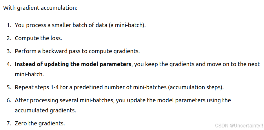 gradient accumulation.jpg |
Key Points
1.Batch Size vs. Mini-Batch Size:
(1) The original batch size is split into smaller mini-batches to fit into GPU memory.
(2) accumulation_steps * mini_batch_size = effective_batch_size.
2.Loss Scaling:
(1) The loss is divided by accumulation_steps to ensure that the gradient magnitudes remain consistent with what they would be if you processed the entire batch at once.
3.Optimizer Step and Gradient Zeroing:
(1) The optimizer step is performed, and gradients are zeroed only after accumulating gradients over several mini-batches.
from torch.cuda.amp import GradScaler, autocast# Assuming you have defined your model, optimizer, loss function, and data loader
model = UNET().to(device)
optimizer = optim.AdamW(model.parameters(), lr=args.lr)
scaler = GradScaler()
mse = nn.MSELoss()
accumulation_steps = 4  # Number of mini-batches to accumulate gradients overfor epoch in range(args.epochs):model.train()optimizer.zero_grad()for batch_idx, (images, captions) in enumerate(train_loader):images = images.to(device)captions = captions.to(device)text_embeddings = torch.squeeze(captions, dim=1)timesteps = ddpm_sampler.sample_timesteps(images.shape[0]).to(device)noisy_latent_images, noises = ddpm_sampler.add_noise(images, timesteps)time_embeddings = timesteps_to_time_emb(timesteps)with autocast():last_decoder_noise = model(noisy_latent_images, text_embeddings, time_embeddings)final_output = diffusion.final.to(device)predicted_noise = final_output(last_decoder_noise).to(device)loss = mse(noises, predicted_noise) / accumulation_stepsscaler.scale(loss).backward()# Accumulate gradients but do not update the weights yetif (batch_idx + 1) % accumulation_steps == 0:scaler.step(optimizer)scaler.update()optimizer.zero_grad()# Optional: Save model checkpoint after each epochtorch.save(model.state_dict(), f"model_epoch_{epoch}.pth")
2.2.4 Clear Cache
Manually clear the GPU cache to free up unused memory.
from torch.cuda.amp import GradScaler, autocastdef train(args):device = args.devicemodel = UNET().to(device)model.train()optimizer = optim.AdamW(model.parameters(), lr=args.lr)scaler = GradScaler()mse = nn.MSELoss()logger = SummaryWriter(os.path.join("runs", args.run_name))len_train = len(train_loader)for epoch in range(args.epochs):logging.info(f"Starting epoch {epoch}:")progress_bar = tqdm(train_loader)optimizer.zero_grad()accumulation_steps = 4for batch_idx, (images, captions) in enumerate(progress_bar):images = images.to(device)images = torch.squeeze(images, dim=1)captions = captions.to(device)text_embeddings = torch.squeeze(captions, dim=1)timesteps = ddpm_sampler.sample_timesteps(images.shape[0]).to(device)noisy_latent_images, noises = ddpm_sampler.add_noise(images, timesteps)time_embeddings = timesteps_to_time_emb(timesteps)with autocast():last_decoder_noise = model(noisy_latent_images, text_embeddings, time_embeddings)final_output = diffusion.final.to(device)predicted_noise = final_output(last_decoder_noise).to(device)loss = mse(noises, predicted_noise) / accumulation_stepsscaler.scale(loss).backward()if (batch_idx + 1) % accumulation_steps == 0:scaler.step(optimizer)scaler.update()optimizer.zero_grad()# Clear cache to free up memorytorch.cuda.empty_cache()progress_bar.set_postfix(MSE=loss.item())logger.add_scalar("MSE", loss.item(), global_step=epoch * len_train + batch_idx)# Save model checkpoint after each epochos.makedirs(os.path.join("models", args.run_name), exist_ok=True)torch.save(model.state_dict(), os.path.join("models", args.run_name, f"stable_diffusion.ckpt"))torch.save(optimizer.state_dict(), os.path.join("models", args.run_name, f"optim.pt"))相关文章:
Training for Stable Diffusion
1.Training for Stable Diffusion 笔记来源: 1.Denoising Diffusion Probabilistic Models 2.最大似然估计(Maximum likelihood estimation) 3.Understanding Maximum Likelihood Estimation 4.How to Solve ‘CUDA out of memory’ in PyTorch 5.pytorch-stable-d…...
初学51单片机之指针基础与串口通信应用
开始之前推荐一个电路学习软件,这个软件笔者也刚接触。名字是Circuit有在线版本和不在线版本,这是笔者在B站看视频翻到的。 Paul Falstadhttps://www.falstad.com/这是地址。 离线版本在网站内点这个进去 根据你的系统下载你需要的版本红线的是windows…...

【启明智显分享】甲醛检测仪HMI方案:ESP32-S3方案4.3寸触摸串口屏,RS485、WIFI/蓝牙可选
今年,“串串房”一词频繁引发广大网友关注。“串串房”,也被称为“陷阱房”“贩子房”——炒房客以低价收购旧房子或者毛坯房,用极度节省成本的方式对房子进行装修,之后作为精修房高价租售,因甲醛等有害物质含量极高&a…...

Linux 驱动学习笔记
1、驱动程序分为几类? • 内核驱动程序(Kernel Drivers):这些是运行在操作系统内核空间的驱动程序,用于直接访问和控制硬件设备。它们提供了与硬件交互的底层功能,如处理中断、访问寄存器、数据传输等。 •…...

ip地址设置了重启又改变了怎么回事
在数字世界的浩瀚星海中,IP地址就如同每个设备的“身份证”,确保它们在网络中准确无误地定位与通信。然而,当我们精心为设备配置好IP地址后,却时常遭遇一个令人费解的现象:一旦设备重启,原本设定的IP地址竟…...

layui table 浮动操作内容收缩,展开
layui table 隐藏浮动操作内容 fixed: right, style:, title: 操作,align:left, minWidth: 450, toolbar:#id分析: 浮动一块新增一个class layui-table-fixed-r 可以隐藏整块内容进行,新增一个按钮点击时间,然后进行收缩和展开 $(‘.layui-…...
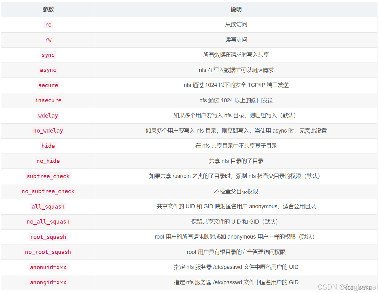
Ubuntu24.04 NFS 服务配置
1、NFS 介绍 NFS 是 Network FileSystem 的缩写,顾名思义就是网络文件存储系统,它允许网络中的计算机之间通过 TCP/IP 网络共享资源。通过 NFS,我们本地 NFS 的客户端应用可以透明地读写位于服务端 NFS 服务器上的文件,就像访问本…...
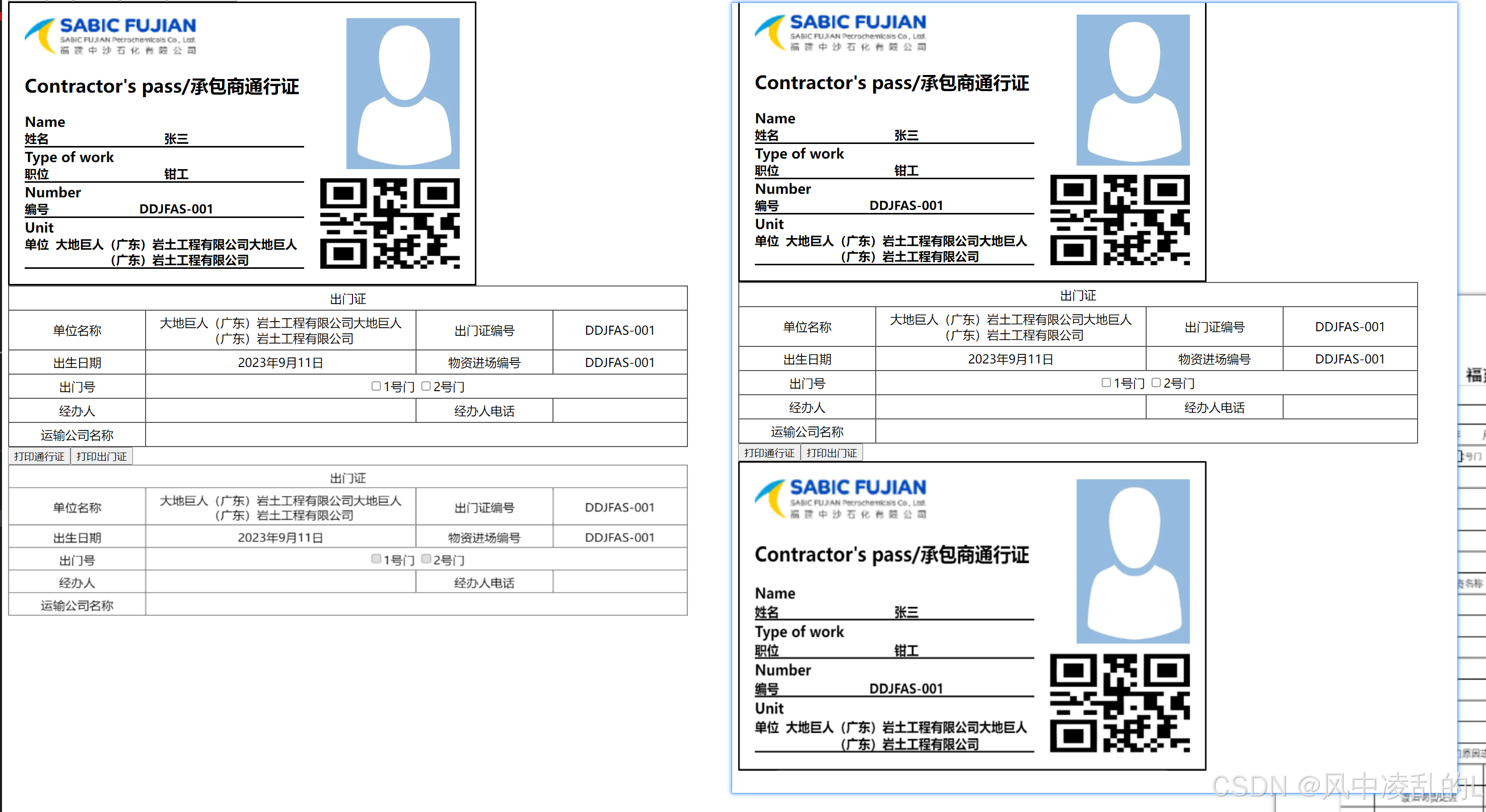
vue3使用html2canvas
安装 yarn add html2canvas 代码 <template><div class"container" ref"container"><div class"left"><img :src"logo" alt"" class"logo"><h2>Contractors pass/承包商通行证&l…...

OpenCV分水岭算法watershed函数的使用
操作系统:ubuntu22.04 OpenCV版本:OpenCV4.9 IDE:Visual Studio Code 编程语言:C11 描述 我们将学会使用基于标记的分水岭算法来进行图像分割。我们将看到:watershed()函数的用法。 任何灰度图像都可以被视为一个地形表…...
laravel为Model设置全局作用域
如果一个项目中存在这么一个sql条件在任何情况下或大多数情况都会被使用,同时很容易被开发者遗忘,那么就非常适用于今天要提到的这个功能,Eloquent\Model的全局作用域。 首先看一个示例,有个数据表,结构如下࿱…...

Leetcode之string
目录 前言1. 字符串相加2. 仅仅反转字母3. 字符串中的第一个唯一字符4. 字符串最后一个单词的长度5. 验证回文串6. 反转字符串Ⅱ7. 反转字符串的单词Ⅲ8. 字符串相乘9. 打印日期 前言 本篇整理了一些关于string类题目的练习, 希望能够学以巩固. 博客主页: 酷酷学!!! 点击关注…...
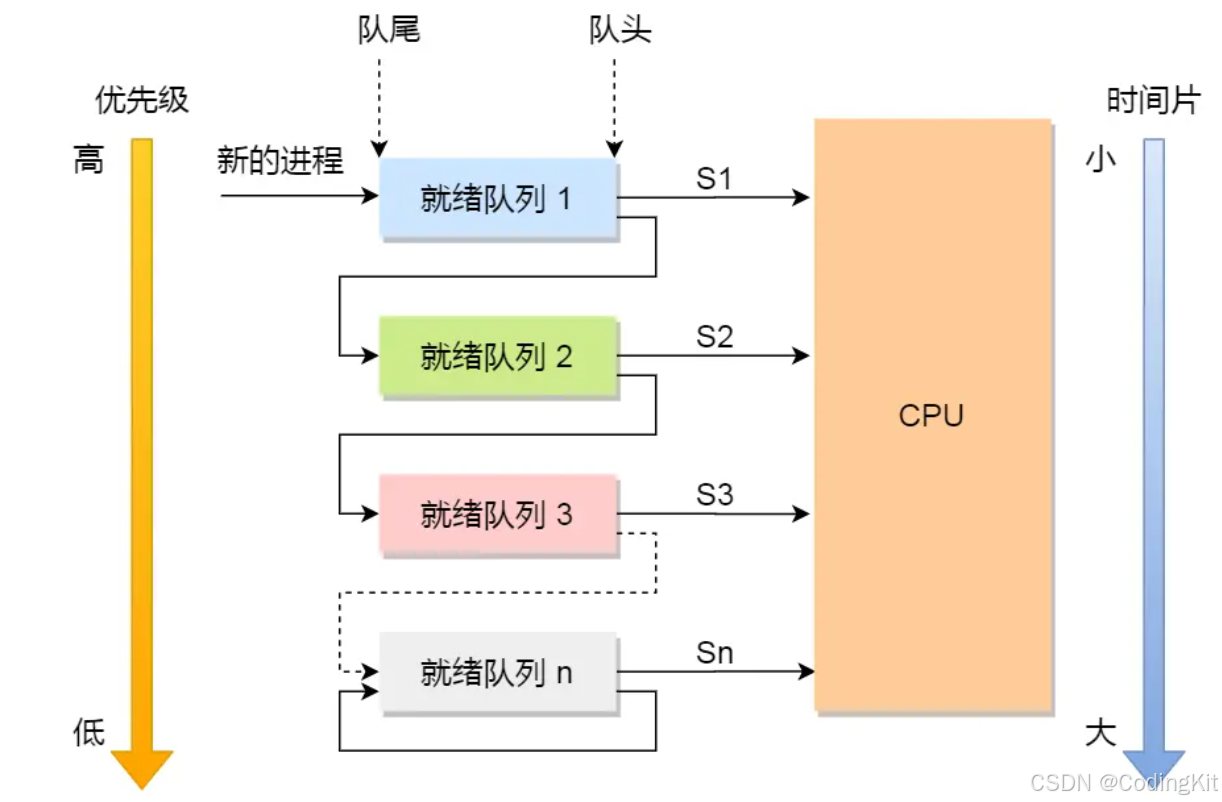
OS:处理机进程调度
1.BackGround:为什么要进行进程调度? 在多进程环境下,内存中存在着多个进程,其数目往往多于处理机核心数目。这就要求系统可以按照某种算法,动态的将处理机CPU资源分配给处于就绪状态的进程。调度算法的实质其实是一种…...
——DBSCAN算法)
【车辆轨迹处理】python实现轨迹点的聚类(一)——DBSCAN算法
提示:文章写完后,目录可以自动生成,如何生成可参考右边的帮助文档 文章目录 前言一、单辆车轨迹的聚类与分析1.引入库2.聚类3.聚类评价 二、整个数据集多辆车聚类1.聚类2.整体评价 前言 空间聚类是基于一定的相似性度量对空间大数据集进行分组…...

Apache Kylin
Apache Kylin 是一个开源的分布式分析引擎,提供 SQL 查询接口及多维分析(OLAP)能力以支持超大规模数据集。它能在亚秒级的时间内提供 PB 级数据的查询能力,非常适合大数据分析和报表系统。 ### 入门指南 #### 1. 环境准备 首先…...

为何Vue3比Vue2快
Proxy响应式 PatchFlag 编译模板时,动态节点做标记标记,分为不同的类型,如TEXT PROPSdiff算法时,可以区分静态节点,以及不同类型的动态节点 <div>Hello World</div> <span>{{ msg }}</span>…...

人工智能与社交变革:探索Facebook如何领导智能化社交平台
在过去十年中,人工智能(AI)技术迅猛发展,彻底改变了我们与数字世界互动的方式。Facebook作为全球最大的社交媒体平台之一,充分利用AI技术,不断推动社交平台的智能化,提升用户体验。本文将深入探…...

八股文之java基础
jdk9中对字符串进行了一个什么优化? jdk9之前 字符串的拼接通常都是使用进行拼接 但是的实现我们是基于stringbuilder进行的 这个过程通常比较低效 包含了创建stringbuilder对象 通过append方法去将stringbuilder对象进行拼接 最后使用tostring方法去转换成最终的…...
深度挖掘行情接口:股票市场中的关键金融数据API接口解析
在股票市场里,存在若干常见的股票行情数据接口,每一种接口皆具备独特的功能与用途。以下为一些常见的金融数据 API 接口,其涵盖了广泛的金融数据内容,其中就包含股票行情数据: 实时行情接口 实时行情接口:…...

逆向破解 对汇编的 简单思考
逆向破解汇编非常之简单 只是一些反逆向技术非常让人难受 但网络里都有方法破解 申请变量 : int a 0; 00007FF645D617FB mov dword ptr [a],0 char b b; 00007FF645D61802 mov byte ptr [b],62h double c 0.345; 00007FF645D61…...

搜维尔科技:人机交互学术应用概览
人机交互学术应用概览 搜维尔科技:人机交互学术应用概览...

深入解析SD卡CMD指令集:从寄存器操作到数据传输实战
1. SD卡基础寄存器全解析 当你把一张SD卡插入读卡器时,系统瞬间就能识别出容量和型号,这个过程背后其实是SD卡内部寄存器的功劳。这些寄存器就像SD卡的"身份证"和"体检报告",存储着所有关键信息。我刚开始接触嵌入式开发…...

5步搞定Qwen3-ASR语音识别:支持多语言和方言,快速上手教程
5步搞定Qwen3-ASR语音识别:支持多语言和方言,快速上手教程 语音识别技术正在改变我们与数字世界的交互方式,而Qwen3-ASR以其强大的多语言和方言支持能力脱颖而出。本文将带你用最简单的方式,在5个步骤内完成这个专业级语音识别系…...

旧设备重生:如何让经典iOS设备突破系统限制重获新生?
旧设备重生:如何让经典iOS设备突破系统限制重获新生? 【免费下载链接】Legacy-iOS-Kit An all-in-one tool to downgrade/restore, save SHSH blobs, and jailbreak legacy iOS devices 项目地址: https://gitcode.com/gh_mirrors/le/Legacy-iOS-Kit …...
)
跨地域公司短号互拨实战:用miniSIPServer+SIP话机打通两地分机(含完整号码变换规则)
跨地域企业短号互通实战:基于miniSIPServer的智能路由与号码变换体系 当企业分支机构分布在不同城市时,如何让员工继续沿用熟悉的短号拨号习惯,同时实现主叫号码的规范显示?这个看似简单的需求背后,隐藏着VoIP系统中号…...

MOOTDX:Python通达信数据接口解决方案
MOOTDX:Python通达信数据接口解决方案 【免费下载链接】mootdx 通达信数据读取的一个简便使用封装 项目地址: https://gitcode.com/GitHub_Trending/mo/mootdx 在量化投资领域,数据获取与处理始终是从业者面临的核心挑战。个人投资者常常困于复杂…...

WarcraftHelper:魔兽争霸3兼容性问题的全方位解决方案
WarcraftHelper:魔兽争霸3兼容性问题的全方位解决方案 【免费下载链接】WarcraftHelper Warcraft III Helper , support 1.20e, 1.24e, 1.26a, 1.27a, 1.27b 项目地址: https://gitcode.com/gh_mirrors/wa/WarcraftHelper 问题发现:现代系统下的经…...

Fun-ASR-MLT-Nano-2512在教育培训场景的应用:语音课件自动转写
Fun-ASR-MLT-Nano-2512在教育培训场景的应用:语音课件自动转写 1. 技术背景与教育痛点 1.1 教育培训行业的语音处理需求 教育培训行业每天产生大量语音内容,包括教师授课录音、在线课程音频、学生互动语音等。传统的人工转写方式面临三大核心痛点&…...

数据救援3大维度全解析:开源工具TestDisk PhotoRec实战指南
数据救援3大维度全解析:开源工具TestDisk & PhotoRec实战指南 【免费下载链接】testdisk TestDisk & PhotoRec 项目地址: https://gitcode.com/gh_mirrors/te/testdisk 硬盘数据恢复是每个技术人员都可能面临的挑战,当遭遇分区损坏、文件…...
与内部IRC40K)
保姆级教程:手把手配置GD32的RTC外部低速时钟(LXTAL)与内部IRC40K
GD32 RTC时钟源配置实战:从LXTAL到IRC40K的深度解析 在嵌入式开发中,实时时钟(RTC)模块的稳定运行往往决定了设备的时间记录精度和低功耗表现。作为GD32微控制器的重要外设之一,RTC模块支持多种时钟源配置方案,其中外部低速晶振(L…...
ater到实战加固:剖析SSH密钥交换DoS漏洞的攻防演进与缓解策略)
从D(HE)ater到实战加固:剖析SSH密钥交换DoS漏洞的攻防演进与缓解策略
1. 当SSH握手变成CPU绞肉机:D(HE)ater攻击原理拆解 那天凌晨三点,运维老张被刺耳的告警声惊醒。监控大屏上,十几台服务器的CPU曲线全部飙到100%,而罪魁祸首竟然是看似无害的SSH服务。这就是典型的D(HE)ater攻击现场——攻击者用特…...