错误修改系列---基于RNN模型的心脏病预测(pytorch实现)
前言
- 前几天发布了pytorch实现,TensorFlow实现为:基于RNN模型的心脏病预测(tensorflow实现),但是一处繁琐地方 + 一处错误,
这篇文章进行修改,修改效果还是好了不少; - 源文章为:基于RNN模型的心脏病预测,提供tensorflow和pytorch实现
错误一
这个也不算是错误,就是之前数据标准化、划分数据集的时候,我用的很麻烦,如下图(之前):

这样无疑是很麻烦的,修改后,我们先对数据进行标准化,后再进行划分就会简单很多(详细请看下面代码)
错误二
模型参数输入,这里应该是13个特征维度,而且这里用nn.BCELoss后面处理也不好,因为最后应该还加一层激活函数sigmoid的,所以这次修改采用多分类处理方法,激活函数采用CrossEntropyLoss,具体如图:

BCELoss、CrossEntropyLoss参考资料:
https://blog.csdn.net/qq_36803941/article/details/138673111
https://zhuanlan.zhihu.com/p/98785902
https://www.cnblogs.com/zhangxianrong/p/14773075.html
https://zhuanlan.zhihu.com/p/59800597
修改版本代码
1、数据处理
1、导入库
import pandas as pd
import numpy as np
import matplotlib.pyplot as plt
from torch.utils.data import DataLoader, TensorDataset
import torch device = 'cuda' if torch.cuda.is_available() else 'cpu'
device
'cuda'
2、导入数据
data = pd.read_csv('./heart.csv')data.head()
| age | sex | cp | trestbps | chol | fbs | restecg | thalach | exang | oldpeak | slope | ca | thal | target | |
|---|---|---|---|---|---|---|---|---|---|---|---|---|---|---|
| 0 | 63 | 1 | 3 | 145 | 233 | 1 | 0 | 150 | 0 | 2.3 | 0 | 0 | 1 | 1 |
| 1 | 37 | 1 | 2 | 130 | 250 | 0 | 1 | 187 | 0 | 3.5 | 0 | 0 | 2 | 1 |
| 2 | 41 | 0 | 1 | 130 | 204 | 0 | 0 | 172 | 0 | 1.4 | 2 | 0 | 2 | 1 |
| 3 | 56 | 1 | 1 | 120 | 236 | 0 | 1 | 178 | 0 | 0.8 | 2 | 0 | 2 | 1 |
| 4 | 57 | 0 | 0 | 120 | 354 | 0 | 1 | 163 | 1 | 0.6 | 2 | 0 | 2 | 1 |
- age - 年龄
- sex - (1 = male(男性); 0 = (女性))
- cp - chest pain type(胸部疼痛类型)(1:典型的心绞痛-typical,2:非典型心绞痛-atypical,3:没有心绞痛-non-anginal,4:无症状-asymptomatic)
- trestbps - 静息血压 (in mm Hg on admission to the hospital)
- chol - 胆固醇 in mg/dl
- fbs - (空腹血糖 > 120 mg/dl) (1 = true; 0 = false)
- restecg - 静息心电图测量(0:普通,1:ST-T波异常,2:可能左心室肥大)
- thalach - 最高心跳率
- exang - 运动诱发心绞痛 (1 = yes; 0 = no)
- oldpeak - 运动相对于休息引起的ST抑制
- slope - 运动ST段的峰值斜率(1:上坡-upsloping,2:平的-flat,3:下坡-downsloping)
- ca - 主要血管数目(0-4)
- thal - 一种叫做地中海贫血的血液疾病(3 = normal; 6 = 固定的缺陷-fixed defect; 7 = 可逆的缺陷-reversable defect)
- target - 是否患病 (1=yes, 0=no)
3、数据分析
数据初步分析
data.info() # 数据类型分析
<class 'pandas.core.frame.DataFrame'>
RangeIndex: 303 entries, 0 to 302
Data columns (total 14 columns):#   Column    Non-Null Count  Dtype
---  ------    --------------  -----  0   age       303 non-null    int64  1   sex       303 non-null    int64  2   cp        303 non-null    int64  3   trestbps  303 non-null    int64  4   chol      303 non-null    int64  5   fbs       303 non-null    int64  6   restecg   303 non-null    int64  7   thalach   303 non-null    int64  8   exang     303 non-null    int64  9   oldpeak   303 non-null    float6410  slope     303 non-null    int64  11  ca        303 non-null    int64  12  thal      303 non-null    int64  13  target    303 non-null    int64
dtypes: float64(1), int64(13)
memory usage: 33.3 KB
其中分类变量为:sex、cp、fbs、restecg、exang、slope、ca、thal、target
数值型变量:age、trestbps、chol、thalach、oldpeak
data.describe() # 描述性
| age | sex | cp | trestbps | chol | fbs | restecg | thalach | exang | oldpeak | slope | ca | thal | target | |
|---|---|---|---|---|---|---|---|---|---|---|---|---|---|---|
| count | 303.000000 | 303.000000 | 303.000000 | 303.000000 | 303.000000 | 303.000000 | 303.000000 | 303.000000 | 303.000000 | 303.000000 | 303.000000 | 303.000000 | 303.000000 | 303.000000 |
| mean | 54.366337 | 0.683168 | 0.966997 | 131.623762 | 246.264026 | 0.148515 | 0.528053 | 149.646865 | 0.326733 | 1.039604 | 1.399340 | 0.729373 | 2.313531 | 0.544554 |
| std | 9.082101 | 0.466011 | 1.032052 | 17.538143 | 51.830751 | 0.356198 | 0.525860 | 22.905161 | 0.469794 | 1.161075 | 0.616226 | 1.022606 | 0.612277 | 0.498835 |
| min | 29.000000 | 0.000000 | 0.000000 | 94.000000 | 126.000000 | 0.000000 | 0.000000 | 71.000000 | 0.000000 | 0.000000 | 0.000000 | 0.000000 | 0.000000 | 0.000000 |
| 25% | 47.500000 | 0.000000 | 0.000000 | 120.000000 | 211.000000 | 0.000000 | 0.000000 | 133.500000 | 0.000000 | 0.000000 | 1.000000 | 0.000000 | 2.000000 | 0.000000 |
| 50% | 55.000000 | 1.000000 | 1.000000 | 130.000000 | 240.000000 | 0.000000 | 1.000000 | 153.000000 | 0.000000 | 0.800000 | 1.000000 | 0.000000 | 2.000000 | 1.000000 |
| 75% | 61.000000 | 1.000000 | 2.000000 | 140.000000 | 274.500000 | 0.000000 | 1.000000 | 166.000000 | 1.000000 | 1.600000 | 2.000000 | 1.000000 | 3.000000 | 1.000000 |
| max | 77.000000 | 1.000000 | 3.000000 | 200.000000 | 564.000000 | 1.000000 | 2.000000 | 202.000000 | 1.000000 | 6.200000 | 2.000000 | 4.000000 | 3.000000 | 1.000000 |
- 年纪:均值54,中位数55,标准差9,说明主要是老年人,偏大
- 静息血压:均值131.62, 成年人一般:正常血压:收缩压 < 120 mmHg,偏大
- 胆固醇:均值246.26,理想水平:小于 200 mg/dL,偏大
- 最高心率:均值149.64,一般静息状态下通常是 60 到 100 次每分钟,偏大
最大值和最小值都可能发生,无异常值
缺失值
data.isnull().sum()
age         0
sex         0
cp          0
trestbps    0
chol        0
fbs         0
restecg     0
thalach     0
exang       0
oldpeak     0
slope       0
ca          0
thal        0
target      0
dtype: int64
相关性分析
import seaborn as snsplt.figure(figsize=(20, 15))sns.heatmap(data.corr(), annot=True, cmap='Greens')plt.show()

相关系数的等级划分
- 非常弱的相关性:
- 0.00 至 0.19 或 -0.00 至 -0.19
- 解释:几乎不存在线性关系。
- 弱相关性:
- 0.20 至 0.39 或 -0.20 至 -0.39
- 解释:存在一定的线性关系,但较弱。
- 中等相关性:
- 0.40 至 0.59 或 -0.40 至 -0.59
- 解释:有明显的线性关系,但不是特别强。
- 强相关性:
- 0.60 至 0.79 或 -0.60 至 -0.79
- 解释:两个变量之间有较强的线性关系。
- 非常强的相关性:
- 0.80 至 1.00 或 -0.80 至 -1.00
- 解释:几乎完全线性相关,表明两个变量的变化高度一致。
target与chol、没有什么相关性,fbs是分类变量,chol胆固醇是数值型变量,但是从实际角度,这些都有影响,故不剔除特征
4、数据标准化
from sklearn.preprocessing import StandardScalerscaler = StandardScaler()X = data.iloc[:, :-1]
y = data.iloc[:, -1]# 这里只需要对X标准化即可
X = scaler.fit_transform(X)
5、数据划分
这里先划分为:训练集:测试集 = 9:1
from sklearn.model_selection import train_test_split# 由于要使用pytorch,先将数据转化为torch
X = torch.tensor(np.array(X), dtype=torch.float32)
y = torch.tensor(np.array(y), dtype=torch.int64)X_train, X_test, y_train, y_test = train_test_split(X, y, test_size=0.1, random_state=42)# 输出维度
X_train.shape, y_train.shape
(torch.Size([272, 13]), torch.Size([272]))
6、动态加载数据
from torch.utils.data import TensorDataset, DataLoader
train_dl = DataLoader(TensorDataset(X_train, y_train),                       batch_size=64,                        shuffle=True)
test_dl  = DataLoader(TensorDataset(X_test, y_test),                       batch_size=64,                        shuffle=False)
2、创建模型
- 定义一个RNN层
rnn = nn.RNN(input_size=10, hidden_size=20, num_layers=2, nonlinearity=‘tanh’,
bias=True, batch_first=False, dropout=0, bidirectional=False) - input_size: 输入的特征维度
- hidden_size: 隐藏层的特征维度
- num_layers: RNN 层的数量
- nonlinearity: 非线性激活函数 (‘tanh’ 或 ‘relu’)
- bias: 如果为 False,则内部不含偏置项,默认为 True
- batch_first: 如果为 True,则输入和输出张量提供为 (batch, seq, feature),默认为 False (seq, batch, feature)
- dropout: 如果非零,则除了最后一层,在每层的输出中引入一个 Dropout 层,默认为 0
- bidirectional: 如果为 True,则将成为双向 RNN,默认为 False
import torch
import torch.nn as nn # 创建模型
'''
该问题本质是二分类问题,故最后一层全连接层用激活函数为:sigmoid
模型结构:RNN:隐藏层200,激活函数:reluLinear:--> 100(relu) -> 1(sigmoid)
'''
# 创建模型
class Model(nn.Module):def __init__(self):super().__init__()self.rnn = nn.RNN(input_size=13, hidden_size=200, num_layers=1, batch_first=True)self.fc1 = nn.Linear(200, 50)#self.fc2 = nn.Linear(100, 50)self.fc3 = nn.Linear(50, 2)def forward(self, x):x, hidden1 = self.rnn(x)x = self.fc1(x)#x = self.fc2(x)x = self.fc3(x)return xmodel = Model().to(device)
model
Model((rnn): RNN(13, 200, batch_first=True)(fc1): Linear(in_features=200, out_features=50, bias=True)(fc3): Linear(in_features=50, out_features=2, bias=True)
)
# 查看模型输出的维度
model(torch.rand(30,13).to(device)).shape
torch.Size([30, 2])
3、模型训练
1、设置超参数
loss_fn = nn.CrossEntropyLoss()
lr = 1e-4
optimizer = torch.optim.Adam(model.parameters(), lr=lr)
2、设置训练函数
def train(dataloader, model, loss_fn, optimizer):# 总大小size = len(dataloader.dataset)# 批次大小batch_size = len(dataloader)# 准确率和损失trian_acc, train_loss = 0, 0# 训练for X, y in dataloader:X, y = X.to(device), y.to(device)# 模型训练与误差评分pred = model(X)loss = loss_fn(pred, y)# 梯度清零optimizer.zero_grad() # 梯度上更新# 方向传播loss.backward()# 梯度更新optimizer.step()# 记录损失和准确率train_loss += loss.item()trian_acc += (pred.argmax(1) == y).type(torch.float64).sum().item()# 计算损失和准确率trian_acc /= sizetrain_loss /= batch_sizereturn trian_acc, train_loss
3、设置测试函数
def test(dataloader, model, loss_fn):size = len(dataloader.dataset)batch_size = len(dataloader)test_acc, test_loss = 0, 0with torch.no_grad():for X, y in dataloader:X, y = X.to(device), y.to(device)pred = model(X)loss = loss_fn(pred, y)test_loss += loss.item()test_acc += (pred.argmax(1) == y).type(torch.float64).sum().item()test_acc /= size test_loss /= batch_sizereturn test_acc, test_loss
4、模型训练
train_acc = []
train_loss = []
test_acc = []
test_loss = []# 定义训练次数
epoches = 50for epoch in range(epoches):# 训练model.train()epoch_trian_acc, epoch_train_loss = train(train_dl, model, loss_fn, optimizer)# 测试model.eval()epoch_test_acc, epoch_test_loss = test(test_dl, model, loss_fn)# 记录train_acc.append(epoch_trian_acc)train_loss.append(epoch_train_loss)test_acc.append(epoch_test_acc)test_loss.append(epoch_test_loss)template = ('Epoch:{:2d}, Train_acc:{:.1f}%, Train_loss:{:.3f}, Test_acc:{:.1f}%, Test_loss:{:.3f}')print(template.format(epoch+1, epoch_trian_acc*100, epoch_train_loss, epoch_test_acc*100, epoch_test_loss))
Epoch: 1, Train_acc:49.6%, Train_loss:0.686, Test_acc:58.1%, Test_loss:0.684
Epoch: 2, Train_acc:62.1%, Train_loss:0.682, Test_acc:64.5%, Test_loss:0.671
Epoch: 3, Train_acc:68.0%, Train_loss:0.662, Test_acc:71.0%, Test_loss:0.658
Epoch: 4, Train_acc:69.1%, Train_loss:0.655, Test_acc:77.4%, Test_loss:0.645
Epoch: 5, Train_acc:73.9%, Train_loss:0.643, Test_acc:80.6%, Test_loss:0.632
Epoch: 6, Train_acc:74.3%, Train_loss:0.637, Test_acc:80.6%, Test_loss:0.620
Epoch: 7, Train_acc:75.7%, Train_loss:0.620, Test_acc:80.6%, Test_loss:0.608
Epoch: 8, Train_acc:78.3%, Train_loss:0.612, Test_acc:80.6%, Test_loss:0.596
Epoch: 9, Train_acc:79.8%, Train_loss:0.591, Test_acc:83.9%, Test_loss:0.586
Epoch:10, Train_acc:79.0%, Train_loss:0.590, Test_acc:83.9%, Test_loss:0.575
Epoch:11, Train_acc:81.2%, Train_loss:0.584, Test_acc:83.9%, Test_loss:0.563
Epoch:12, Train_acc:79.8%, Train_loss:0.562, Test_acc:83.9%, Test_loss:0.553
Epoch:13, Train_acc:80.5%, Train_loss:0.546, Test_acc:83.9%, Test_loss:0.542
Epoch:14, Train_acc:80.1%, Train_loss:0.546, Test_acc:83.9%, Test_loss:0.531
Epoch:15, Train_acc:81.2%, Train_loss:0.517, Test_acc:83.9%, Test_loss:0.521
Epoch:16, Train_acc:81.6%, Train_loss:0.521, Test_acc:83.9%, Test_loss:0.509
Epoch:17, Train_acc:82.4%, Train_loss:0.508, Test_acc:83.9%, Test_loss:0.497
Epoch:18, Train_acc:82.7%, Train_loss:0.494, Test_acc:83.9%, Test_loss:0.487
Epoch:19, Train_acc:83.1%, Train_loss:0.496, Test_acc:83.9%, Test_loss:0.477
Epoch:20, Train_acc:82.4%, Train_loss:0.469, Test_acc:83.9%, Test_loss:0.469
Epoch:21, Train_acc:83.1%, Train_loss:0.472, Test_acc:83.9%, Test_loss:0.463
Epoch:22, Train_acc:82.4%, Train_loss:0.451, Test_acc:83.9%, Test_loss:0.458
Epoch:23, Train_acc:83.5%, Train_loss:0.456, Test_acc:83.9%, Test_loss:0.455
Epoch:24, Train_acc:83.1%, Train_loss:0.438, Test_acc:83.9%, Test_loss:0.453
Epoch:25, Train_acc:83.5%, Train_loss:0.431, Test_acc:80.6%, Test_loss:0.451
Epoch:26, Train_acc:84.2%, Train_loss:0.444, Test_acc:80.6%, Test_loss:0.449
Epoch:27, Train_acc:83.1%, Train_loss:0.427, Test_acc:80.6%, Test_loss:0.449
Epoch:28, Train_acc:84.2%, Train_loss:0.409, Test_acc:80.6%, Test_loss:0.449
Epoch:29, Train_acc:83.8%, Train_loss:0.405, Test_acc:80.6%, Test_loss:0.448
Epoch:30, Train_acc:83.8%, Train_loss:0.411, Test_acc:80.6%, Test_loss:0.448
Epoch:31, Train_acc:83.8%, Train_loss:0.378, Test_acc:80.6%, Test_loss:0.446
Epoch:32, Train_acc:84.6%, Train_loss:0.421, Test_acc:80.6%, Test_loss:0.444
Epoch:33, Train_acc:84.6%, Train_loss:0.391, Test_acc:80.6%, Test_loss:0.443
Epoch:34, Train_acc:85.7%, Train_loss:0.388, Test_acc:80.6%, Test_loss:0.446
Epoch:35, Train_acc:84.2%, Train_loss:0.396, Test_acc:80.6%, Test_loss:0.449
Epoch:36, Train_acc:84.2%, Train_loss:0.346, Test_acc:80.6%, Test_loss:0.451
Epoch:37, Train_acc:84.9%, Train_loss:0.379, Test_acc:80.6%, Test_loss:0.453
Epoch:38, Train_acc:84.9%, Train_loss:0.389, Test_acc:80.6%, Test_loss:0.453
Epoch:39, Train_acc:83.1%, Train_loss:0.386, Test_acc:80.6%, Test_loss:0.453
Epoch:40, Train_acc:84.9%, Train_loss:0.350, Test_acc:80.6%, Test_loss:0.452
Epoch:41, Train_acc:83.5%, Train_loss:0.353, Test_acc:80.6%, Test_loss:0.455
Epoch:42, Train_acc:85.7%, Train_loss:0.373, Test_acc:80.6%, Test_loss:0.458
Epoch:43, Train_acc:84.6%, Train_loss:0.345, Test_acc:80.6%, Test_loss:0.459
Epoch:44, Train_acc:85.3%, Train_loss:0.377, Test_acc:80.6%, Test_loss:0.461
Epoch:45, Train_acc:85.7%, Train_loss:0.354, Test_acc:80.6%, Test_loss:0.462
Epoch:46, Train_acc:84.9%, Train_loss:0.327, Test_acc:80.6%, Test_loss:0.467
Epoch:47, Train_acc:82.7%, Train_loss:0.347, Test_acc:80.6%, Test_loss:0.470
Epoch:48, Train_acc:84.6%, Train_loss:0.350, Test_acc:80.6%, Test_loss:0.470
Epoch:49, Train_acc:84.9%, Train_loss:0.344, Test_acc:80.6%, Test_loss:0.470
Epoch:50, Train_acc:85.3%, Train_loss:0.375, Test_acc:80.6%, Test_loss:0.472
5、结果展示
import matplotlib.pyplot as plt
#隐藏警告
import warnings
warnings.filterwarnings("ignore")               #忽略警告信息
plt.rcParams['font.sans-serif']    = ['SimHei'] # 用来正常显示中文标签
plt.rcParams['axes.unicode_minus'] = False      # 用来正常显示负号
plt.rcParams['figure.dpi']         = 100        #分辨率epoch_length = range(epoches)plt.figure(figsize=(12, 3))plt.subplot(1, 2, 1)
plt.plot(epoch_length, train_acc, label='Train Accuaray')
plt.plot(epoch_length, test_acc, label='Test Accuaray')
plt.legend(loc='lower right')
plt.title('Accurary')plt.subplot(1, 2, 2)
plt.plot(epoch_length, train_loss, label='Train Loss')
plt.plot(epoch_length, test_loss, label='Test Loss')
plt.legend(loc='upper right')
plt.title('Loss')plt.show()
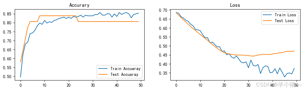
趋于平稳不是没有变化,是变化很小,整体模型效果还可以
6、模型评估
# 评估:返回的是自己在model.compile中设置,这里为accuracy
test_acc, test_loss = test(test_dl, model, loss_fn)
print("socre[loss, accuracy]: ", test_acc, test_loss) # 返回为两个,一个是loss,一个是accuracy
socre[loss, accuracy]: 0.8064516129032258 0.47150832414627075
相关文章:
错误修改系列---基于RNN模型的心脏病预测(pytorch实现)
前言 前几天发布了pytorch实现,TensorFlow实现为:基于RNN模型的心脏病预测(tensorflow实现),但是一处繁琐地方 一处错误,这篇文章进行修改,修改效果还是好了不少;源文章为:基于RNN模型的心脏病…...
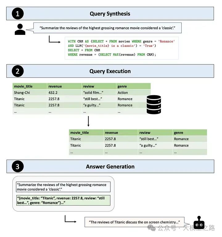
Table-Augmented Generation(TAG):Text2SQL与RAG的升级与超越
当下AI与数据库的融合已成为推动数据管理和分析领域发展的重要力量。传统的数据库查询方式,如结构化查询语言(SQL),要求用户具备专业的数据库知识,这无疑限制了非专业人士对数据的访问和利用。为了打破这一壁垒&#x…...
)
Stable Diffusion本地部署教程(附安装包)
想使用Stable Diffusion需要的环境有哪些呢? python3.10.11(至少也得3.10.6以上):依赖python环境NVIDIA:GPUgit:从github上下载包(可选,由于我已提供安装包,你可以不用git)Stable Diffusion安装包工具包: NVIDIA:https://developer.nvidia.com/cuda-toolkit-archiv…...

【物联网原理与运用】知识点总结(上)
目录 名词解释汇总 第一章 物联网概述 1.1物联网的基本概念及演进 1.2 物联网的内涵 1.3 物联网的特性——泛在性 1.4 物联网的基本特征与属性(五大功能域) 1.5 物联网的体系结构 1.6 物联网的关键技术 1.7 物联网的应用领域 第二章 感知与识别技术 2.1 …...

JuiceFS 2024:开源与商业并进,迈向 AI 原生时代
即将过去的 2024 年,是 JuiceFS 开源版本推出的第 4 年,企业版的第 8 个年头。回顾过去这一年,JuiceFS 社区版依旧保持着快速成长的势头,GitHub 星标突破 11.1K,各项使用指标增长均超过 100%,其中文件系统总…...

C#,动态规划问题中基于单词搜索树(Trie Tree)的单词断句分词( Word Breaker)算法与源代码
1 分词 分词是自然语言处理的基础,分词准确度直接决定了后面的词性标注、句法分析、词向量以及文本分析的质量。英文语句使用空格将单词进行分隔,除了某些特定词,如how many,New York等外,大部分情况下不需要考虑分词…...
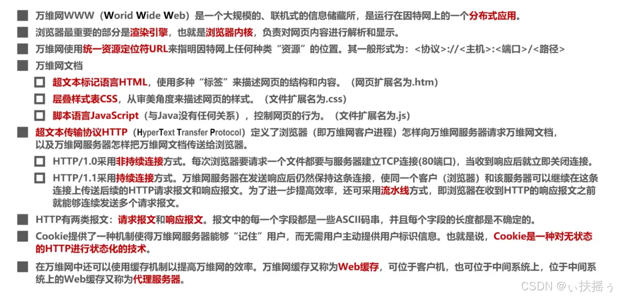
计算机网络(六)应用层
6.1、应用层概述 我们在浏览器的地址中输入某个网站的域名后,就可以访问该网站的内容,这个就是万维网WWW应用,其相关的应用层协议为超文本传送协议HTTP 用户在浏览器地址栏中输入的是“见名知意”的域名,而TCP/IP的网际层使用IP地…...
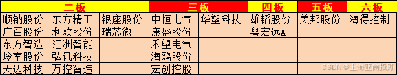
上海亚商投顾:沪指探底回升微涨 机器人概念股午后爆发
上海亚商投顾前言:无惧大盘涨跌,解密龙虎榜资金,跟踪一线游资和机构资金动向,识别短期热点和强势个股。 一.市场情绪 市场全天探底回升,沪指盘中跌超1.6%,创业板指一度跌逾3%,午后集体拉升翻红…...

conda相关操作
conda 是一个开源的包管理和环境管理工具,主要用于 Python 和数据科学领域。它可以帮助用户安装、更新、删除和管理软件包,同时支持创建和管理虚拟环境。以下是关于 conda 的所有常见操作: 1. 安装 Conda Conda 通常通过安装 Anaconda 或 Mi…...

使用TCP协议实现智能聊天机器人
实验目的与要求 本实验是程序设计类实验,要求使用原始套接字编程,掌握TCP/IP协议与网络编程Sockets通信模型,并根据教师给定的任务要求,使用TCP协议实现智能聊天机器人。 (1)熟悉标准库socket 的用法。 …...

PHP二维数组去除重复值
Date: 2025.01.07 20:45:01 author: lijianzhan PHP二维数组内根据ID或者名称去除重复值 代码示例如下: // 假设 data数组如下 $data [[id > 1, name > Type A],[id > 2, name > Type B],[id > 1, name > Type A] // 重复项 ];// 去重方法 $dat…...

2025年01月11日Github流行趋势
项目名称:xiaozhi-esp32 项目地址url:https://github.com/78/xiaozhi-esp32项目语言:C历史star数:2433今日star数:321项目维护者:78, MakerM0, whble, nooodles2023, Kevincoooool项目简介:构建…...
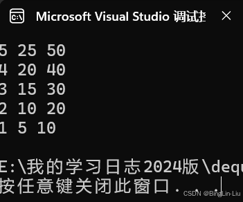
备战蓝桥杯 队列和queue详解
目录 队列的概念 队列的静态实现 总代码 stl的queue 队列算法题 1.队列模板题 2.机器翻译 3.海港 双端队列 队列的概念 和栈一样,队列也是一种访问受限的线性表,它只能在表头位置删除,在表尾位置插入,队列是先进先出&…...

IT面试求职系列主题-Jenkins
想成功求职,必要的IT技能一样不能少,先说说Jenkins的必会知识吧。 1) 什么是Jenkins Jenkins 是一个用 Java 编写的开源持续集成工具。它跟踪版本控制系统,并在发生更改时启动和监视构建系统。 2)Maven、Ant和Jenkins有什么区别…...
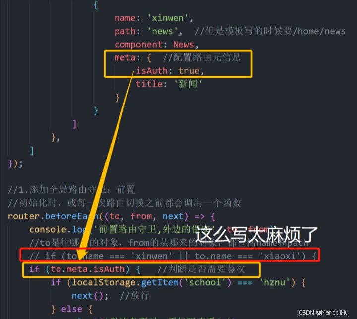
Vue篇-06
1、路由简介 vue-rooter:是vue的一个插件库,专门用来实现SPA应用 1.1、对SPA应用的理解 1、单页 Web 应用(single page web application,SPA)。 2、整个应用只有一个完整的页面 index.html。 3、点击页面中的导航链…...

mysql binlog 日志分析查找
文章目录 前言一、分析 binlog 内容二、编写脚本结果总结 前言 高效快捷分析 mysql binlog 日志文件。 mysql binlog 文件很大 怎么快速通过关键字查找内容 一、分析 binlog 内容 通过 mysqlbinlog 命令可以看到 binlog 解析之后的大概样子 二、编写脚本 编写脚本 search_…...

ubuntu 配置OpenOCD与RT-RT-thread环境的记录
1.git clone git://git.code.sf.net/p/openocd/code openocd 配置gcc编译环境 2. sudo gedit /etc/apt/source.list #cdrom sudo apt-get install git sudo apt-get install libtool-bin sudo apt-get install pkg-config sudo apt-install libusb-1.0-0-dev sudo apt-get…...
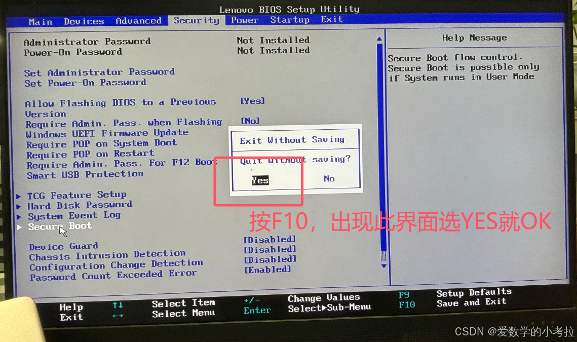
双系统解决开机提示security Policy Violation的方法
最近,Windows系统更新后,发现电脑开机无法进入桌面,显示“Verifiying shim SBAT data failed: security Policy Violation; So mething has gone seriously Wrong: SBAT self-check failed: Security Policy Violation”的英文错误信息。为了…...
的使用场景)
附加共享数据库( ATTACH DATABASE)的使用场景
附加共享数据库(使用 ATTACH DATABASE)的功能非常实用,通常会在以下几种场景下需要用到: 1. 跨数据库查询和分析 场景: 你的公司有两个独立的数据库: 一个存储了学生信息 (school.db)一个存储了员工信息 …...
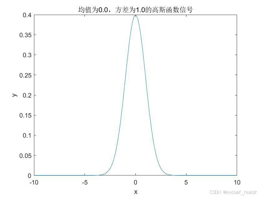
matlab的绘图的标题中(title)添加标量以及格式化输出
有时候我们需要在matlab绘制的图像的标题中添加一些变量,这样在修改某些参数后,标题会跟着一块儿变。可以采用如下的方法: x -10:0.1:10; %x轴的范围 mu 0; %均值 sigma 1; %标准差 y normpdf(x,mu,sigma); %使用normpdf函数生成高斯函数…...

GD32F303实战 ----- 定时器PWM驱动LED实现渐变调光
1. 从零开始理解PWM调光 想象一下老式台灯的旋钮开关,旋转角度越大灯光越亮——这种通过调节"通电时间比例"来控制亮度的原理,就是PWM(脉冲宽度调制)技术的雏形。在GD32F303开发板上,我们通过定时器产生精确…...

D2DX终极指南:如何让经典暗黑破坏神2在现代PC上重获新生?
D2DX终极指南:如何让经典暗黑破坏神2在现代PC上重获新生? 【免费下载链接】d2dx D2DX is a complete solution to make Diablo II run well on modern PCs, with high fps and better resolutions. 项目地址: https://gitcode.com/gh_mirrors/d2/d2dx …...

从选题到成稿:PaperXie AI 期刊写作,让学术发表不再是 “不可能任务”
paperxie-免费查重复率aigc检测/开题报告/毕业论文/智能排版/文献综述/期刊论文https://www.paperxie.cn/ai/journalArticleshttps://www.paperxie.cn/ai/journalArticles 在学术圈,有一句扎心的共识:“写论文难,发期刊更难”。对于本科生、硕…...
中的外点与核函数)
你的SLAM地图为什么“歪”了?深入浅出图解位姿图优化(PGO)中的外点与核函数
为什么你的SLAM地图会"歪斜"?图解位姿图优化中的外点干扰与抗干扰策略 想象一下,你花了整整一周时间搭建的乐高城市,最后发现所有建筑都朝同一个方向微微倾斜——这种崩溃感,和SLAM工程师看到优化后的地图出现系统性偏差…...

uniapp H5 项目实战:集成mui-player实现HLS监控视频流的流畅播放与异常处理
1. 为什么选择mui-player处理HLS监控视频流 在开发监控类H5应用时,视频流的稳定播放是个硬需求。我去年接手过一个智慧园区项目,需要在uniapp里实现多路监控画面的低延迟展示。当时测试了五六种播放方案,最终mui-player以92%的首帧打开率和自…...

STM32 LL库实战:SPI通信的底层驱动与高效轮询
1. STM32 LL库与SPI通信基础 第一次接触STM32的LL库时,我完全被它简洁高效的特性吸引了。相比HAL库,LL库更接近硬件底层,执行效率更高,特别适合对实时性要求严格的场景。记得当时调试一个工业传感器项目,HAL库的延时让…...

AI建站避坑指南:10个高频问题与风险防范方案
随着AI建站工具越来越普及,关于它的疑问和担忧也层出不穷:“AI生成的网站会不会千篇一律,没有品牌特色?”“我的数据和客户资料放在上面安全吗?归谁所有?”“花几千块钱订阅,到底能不能带来效果…...

别再死记硬背了!用D触发器搭个8分频电路,手把手教你理解Verilog时序逻辑
从零构建8分频电路:用D触发器玩转Verilog时序逻辑 第一次接触数字电路设计时,我被各种触发器、寄存器绕得晕头转向。直到导师扔给我一块FPGA开发板:"别光看理论,先搭个分频电路试试"。那次实践让我恍然大悟——原来抽象…...

gh_mirrors/si/simulator扩展开发教程:自定义传感器与车辆模型
gh_mirrors/si/simulator扩展开发教程:自定义传感器与车辆模型 【免费下载链接】simulator A ROS/ROS2 Multi-robot Simulator for Autonomous Vehicles 项目地址: https://gitcode.com/gh_mirrors/si/simulator gh_mirrors/si/simulator是一款专为自动驾驶车…...

03_ONNX Runtime Java:跨框架高性能推理引擎
ONNX Runtime Java:跨框架高性能推理引擎 摘要:ONNX Runtime Java 作为微软官方推出的跨平台推理引擎,为 Java 生态提供了统一接入 PyTorch、TensorFlow、PaddlePaddle 等大模型的能力。本文深入剖析其架构设计、执行提供器机制、性能优化策略…...