MATLAB | 有关数值矩阵、颜色图及颜色列表的技巧整理
这是一篇有关数值矩阵、颜色矩阵、颜色列表的技巧整合,会以随笔的形式想到哪写到哪,可能思绪会比较飘逸请大家见谅,本文大体分为以下几个部分:
- 数值矩阵用颜色显示
- 从颜色矩阵提取颜色
- 从颜色矩阵中提取数据
- 颜色列表相关函数
- 颜色测试图表的识别

数值矩阵用颜色显示
heatmap
我们最常用的肯定就是heatmap函数显示数值矩阵:
X=rand(10);
heatmap(X);
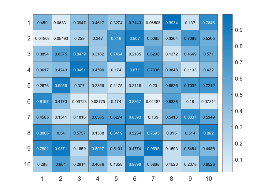
字体颜色可设置为透明:
X=rand(10);
HM=heatmap(X);
HM.CellLabelColor='none';

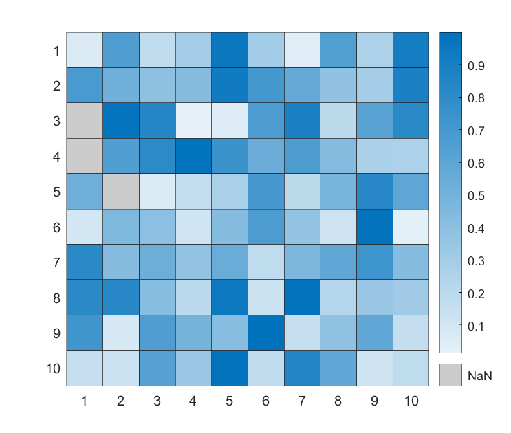
如果由NaN值,会显示为黑色:
X=rand(10);
X([3,4,15])=nan;
HM=heatmap(X);
HM.CellLabelColor='none';

这个颜色也可以改,比如改成浅灰色:
X=rand(10);
X([3,4,15])=nan;
HM=heatmap(X);
HM.CellLabelColor='none';
HM.MissingDataColor=[.8,.8,.8];
imagesc
imagesc随便加个colorbar就和heatmap非常像了,而且比较容易进行图像组合(heatmap的父类不能是axes),但是没有边缘:
X=rand(10);
imagesc(X)
colormap(winter)
colorbar
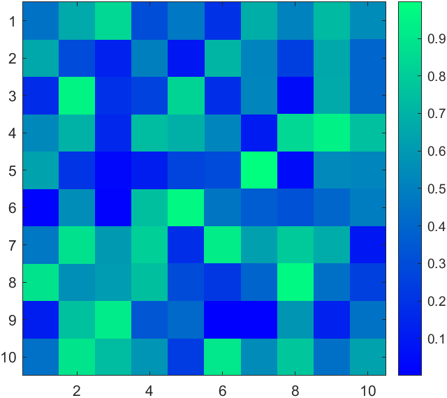
比较烦的是imagesc即使数据有NaN也会对其进行插值显示,好坏参半吧。
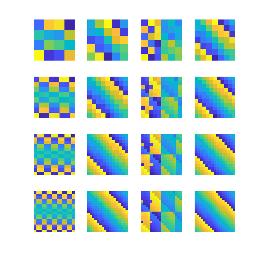
另外随便写了点代码发现MATLAB自带的幻方绘制挺有规律的hiahiahia:
for i=1:16ax=subplot(4,4,i);hold on;axis tight off equalX=magic(3+i);imagesc(X);
end
image
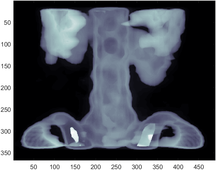
image函数单通道时也可以设置colormap来进行颜色映射:
load spine
image(X)
colormap(map)
pcolor
pcolor由于每个方块颜色都会使用左上角的数值来计算,因此会缺一行一列,我们可以补上一行一列nan:
X=rand(6);
X(end+1,:)=nan;
X(:,end+1)=nan;
pcolor(X);
colormap(winter)
colorbar
可修饰的东西就比较丰富了,比如边缘颜色:
X=rand(6);
X(end+1,:)=nan;
X(:,end+1)=nan;
pHdl=pcolor(X);
pHdl.EdgeColor=[1,1,1];
pHdl.LineWidth=2;
colormap(winter)
colorbar
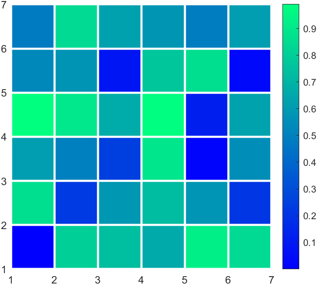
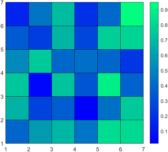
气泡图
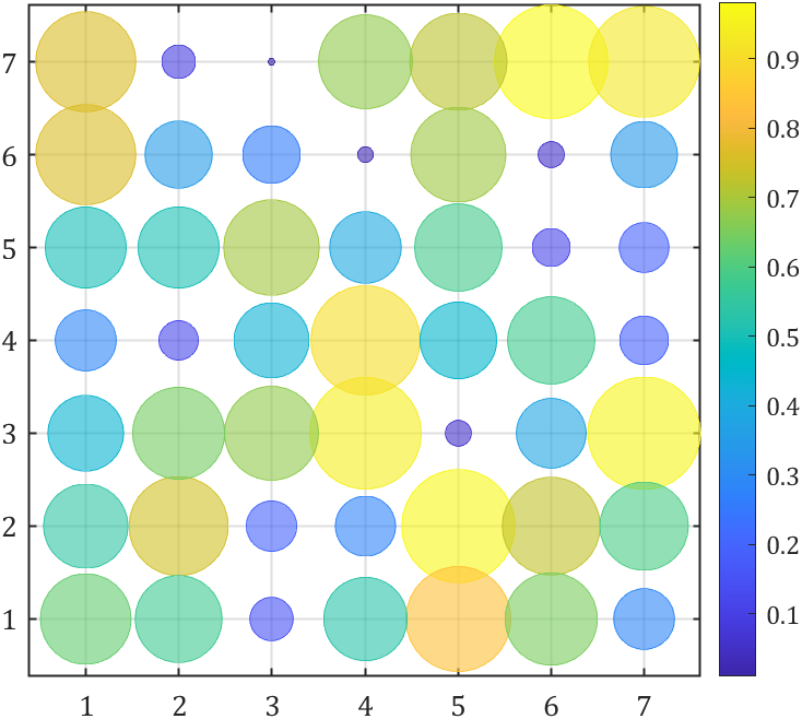
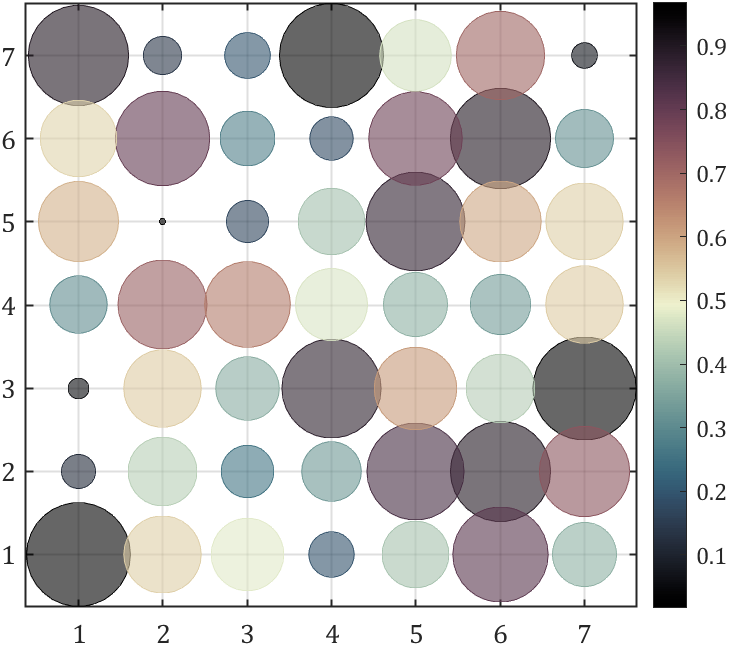
气泡图大概也能冒充一下热图:
Z=rand(7);
[X,Y]=meshgrid(1:size(Z,2),1:size(Z,1));bubblechart(X(:),Y(:),Z(:),Z(:),'MarkerFaceAlpha',.6)
colormap(parula)
colorbar
set(gca,'XTick',1:size(Z,2),'YTick',1:size(Z,1),'LineWidth',1,...'XGrid','on','YGrid','on','FontName','Cambria','FontSize',13)
随便写着玩
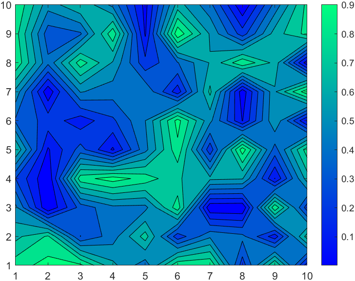
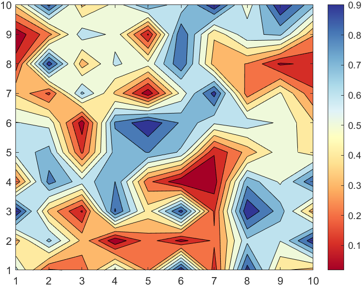
虽然surf函数调整视角也像是热图的样子,但是不打算讲了,反而等高线填充图虽然不像热图但是很有意思,感觉可以当作colormap展示的示例图:
X=rand(10);
CF=contourf(X);
colormap(winter)
colorbar
从颜色矩阵提取颜色
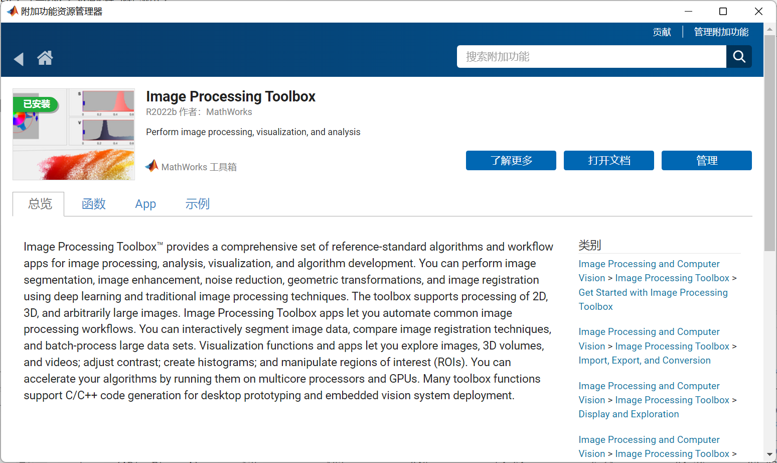
像素提取器
需要安装:
Image Processing Toolbox
图像处理工具箱.
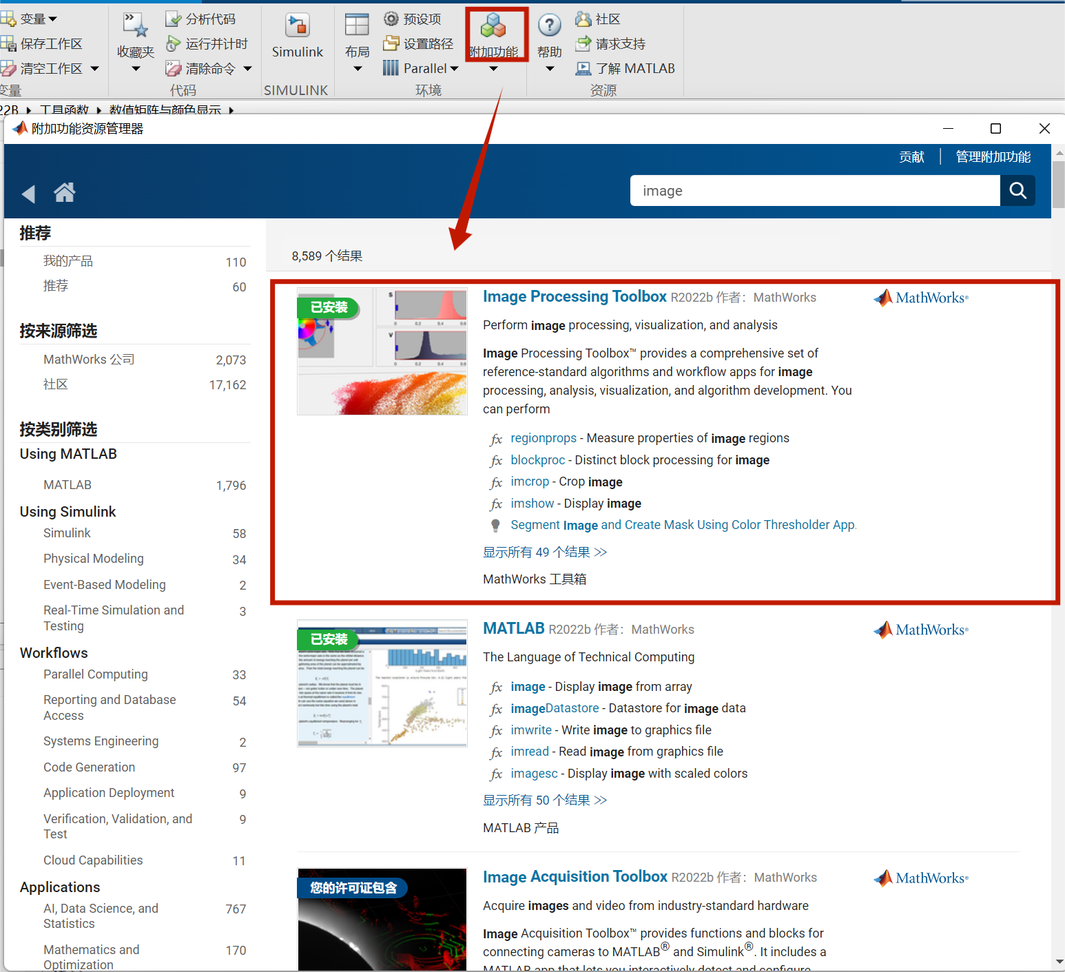
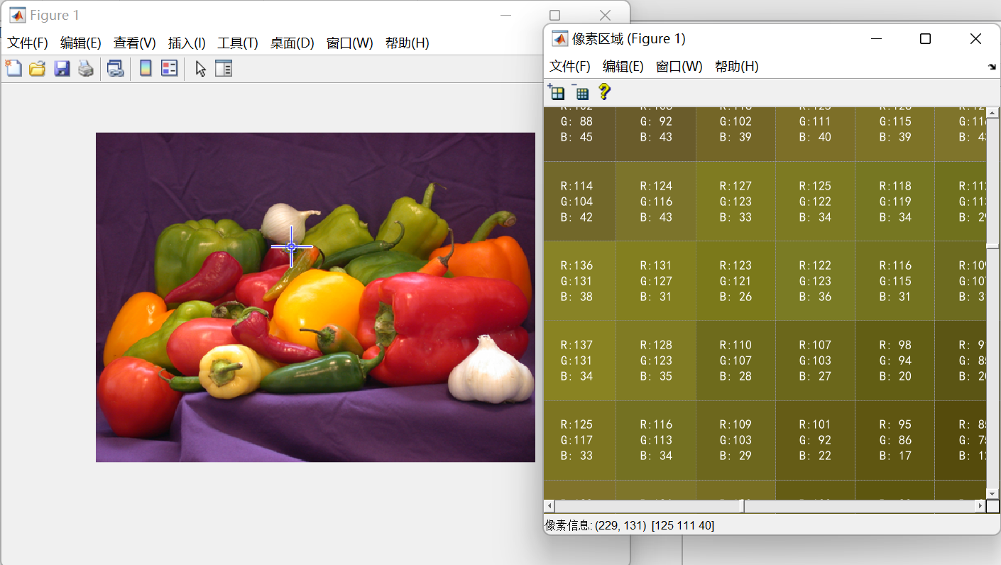
使用以下代码可以显示每个像素RGB值:
imshow('peppers.png')
impixelregion
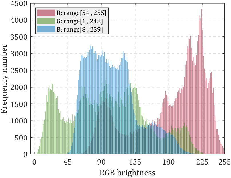
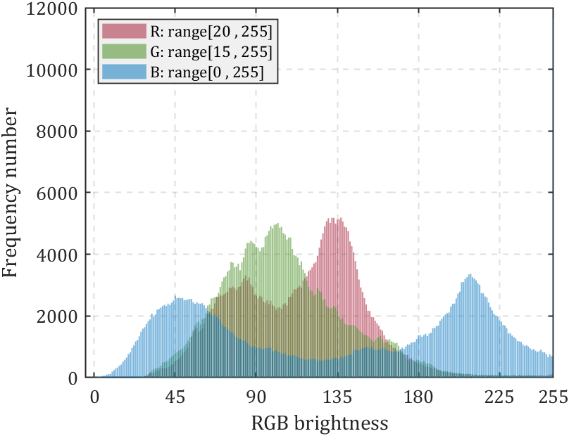
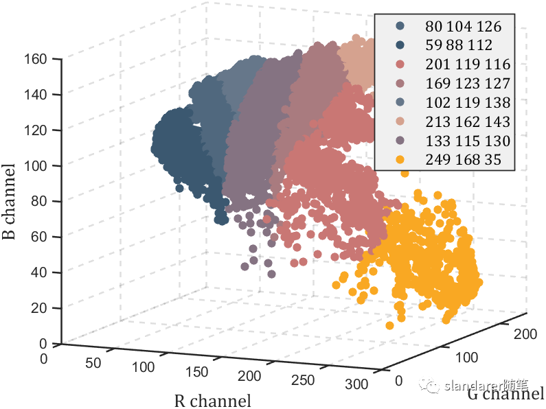
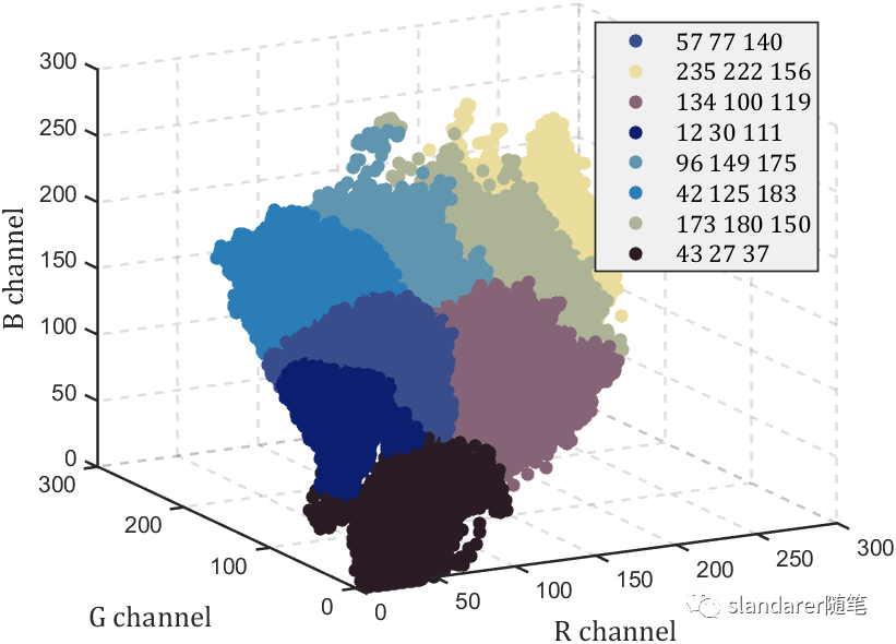
图片颜色统计小函数
我写过一个RGB颜色统计图绘制函数:
function HistogramPic(pic)
FreqNum=zeros(size(pic,3),256);
for i=1:size(pic,3)for j=0:255FreqNum(i,j+1)=sum(sum(pic(:,:,i)==j));end
end
ax=gca;hold(ax,'on');box on;grid on
if size(FreqNum,1)==3bar(0:255,FreqNum(1,:),'FaceColor',[0.6350 0.0780 0.1840],'FaceAlpha',0.5);bar(0:255,FreqNum(2,:),'FaceColor',[0.2400 0.5300 0.0900],'FaceAlpha',0.5);bar(0:255,FreqNum(3,:),'FaceColor',[0 0.4470 0.7410],'FaceAlpha',0.5);ax.XLabel.String='RGB brightness';rrange=[num2str(min(pic(:,:,1),[],[1,2])),' , ',num2str(max(pic(:,:,1),[],[1,2]))];grange=[num2str(min(pic(:,:,2),[],[1,2])),' , ',num2str(max(pic(:,:,2),[],[1,2]))];brange=[num2str(min(pic(:,:,3),[],[1,2])),' , ',num2str(max(pic(:,:,3),[],[1,2]))];legend({['R: range[',rrange,']'],['G: range[',grange,']'],['B: range[',brange,']']},...'Location','northwest','Color',[0.9412 0.9412 0.9412],...'FontName','Cambria','LineWidth',0.8,'FontSize',11);
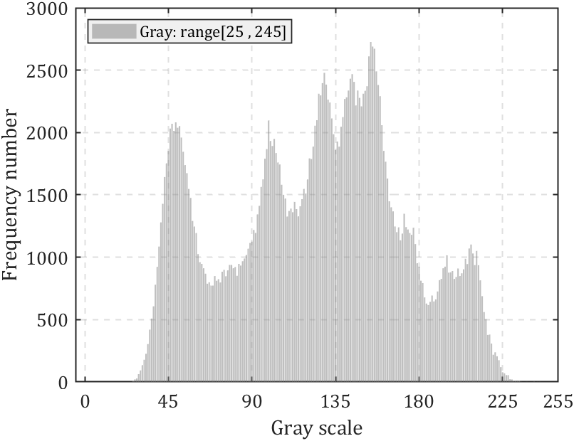
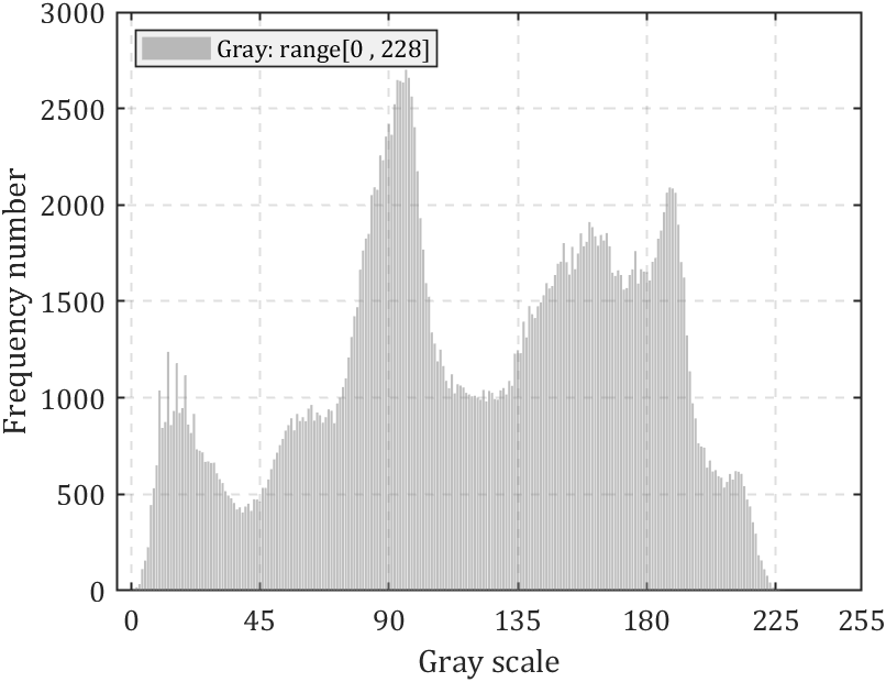
else bar(0:255,FreqNum(1,:),'FaceColor',[0.50 0.50 0.50],'FaceAlpha',0.5);ax.XLabel.String='Gray scale';krange=[num2str(min(pic(:,:,1),[],[1,2])),' , ',num2str(max(pic(:,:,1),[],[1,2]))];legend(['Gray: range[',krange,']'],...'Location','northwest','Color',[0.9412 0.9412 0.9412],...'FontName','Cambria','LineWidth',0.8,'FontSize',11);
end
ax.LineWidth=1;
ax.GridLineStyle='--';
ax.XLim=[-5 255];
ax.XTick=[0:45:255,255];
ax.YLabel.String='Frequency number';
ax.FontName='Cambria';
ax.FontSize=13;
end
非常简单的使用方法,就是读取图片后调用函数即可:
pic=imread('test.png');
HistogramPic(pic)
若图像为灰度图则效果如下:
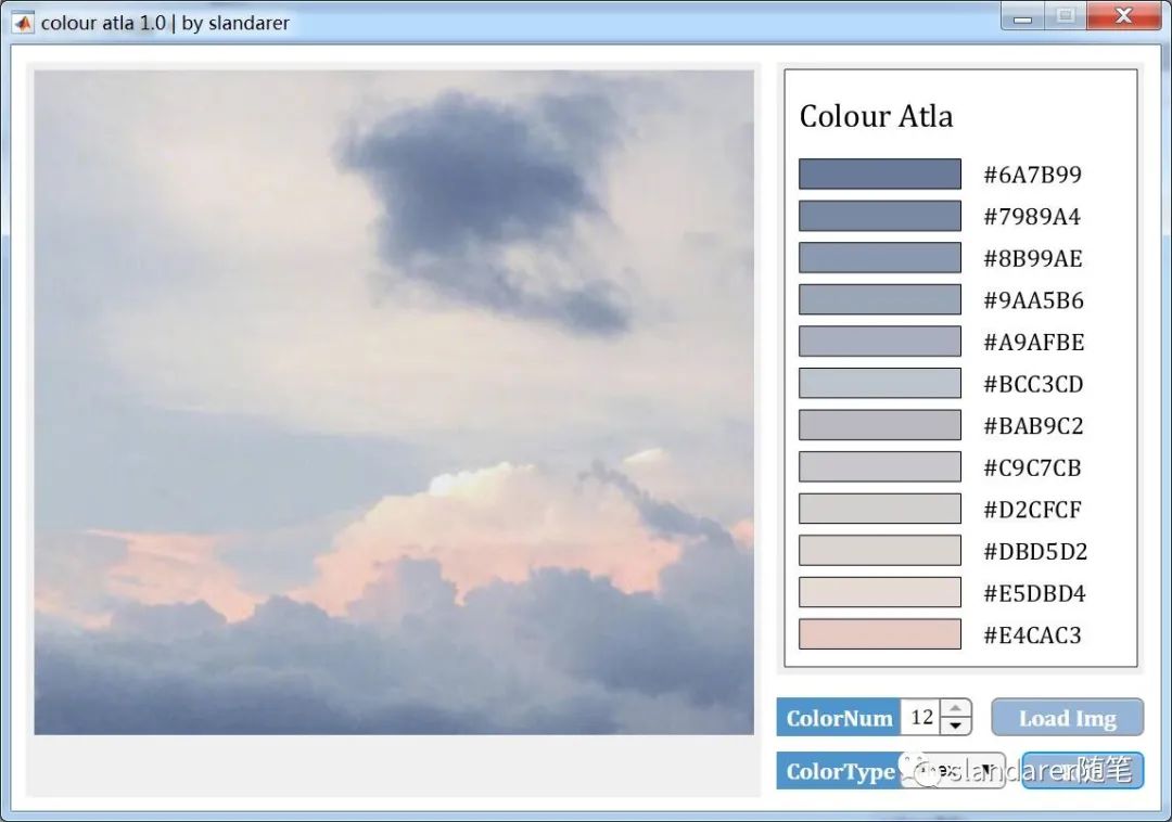
色卡生成器
从图片中提取主要颜色:https://mp.weixin.qq.com/s/Pj6t0SMDBAjQi3ecj6KVaA
颜色提取器
推荐两款颜色提取器,一款免费一款付费:
免费版:https://mp.weixin.qq.com/s/uIyvqQa9Vnz7gYLgd7lUtg
付费版:https://mp.weixin.qq.com/s/BpegP7CpOQERwrUXHexsGQ
从颜色矩阵中提取数据
之前写过一列把热图变为数值矩阵的函数,可以去瞅一眼:https://mp.weixin.qq.com/s/wzqCCFF2yvC80-ruqMKOpQ
颜色列表相关函数
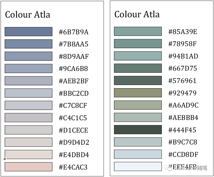
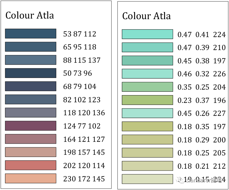
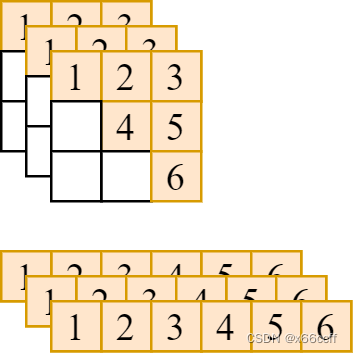
颜色方块展示函数
写了个用来显示颜色的小函数:
function colorSwatches(C,sz)
ax=gca;hold on;
ax.YDir='reverse';
ax.XColor='none';
ax.YColor='none';
ax.DataAspectRatio=[1,1,1];
for i=1:sz(1)for j=1:sz(2)if j+(i-1)*sz(2)<=size(C,1)fill([-.4,-.4,.4,.4]+j,[-.4,.4,.4,-.4]+i,C(j+(i-1)*sz(2),:),...'EdgeColor','none')endend
end
end
使用方式(第一个参数是颜色列表,第二个参数是显示行列数):
C=lines(7);
colorSwatches(C,[3,3])

C=[0.6471         0    0.14900.7778    0.1255    0.15160.8810    0.2680    0.18950.9569    0.4275    0.26270.9804    0.5974    0.34120.9935    0.7477    0.44180.9961    0.8784    0.56470.9987    0.9595    0.68760.9595    0.9843    0.82350.8784    0.9529    0.97250.7399    0.8850    0.93330.5987    0.7935    0.88240.4549    0.6784    0.81960.3320    0.5320    0.74380.2444    0.3765    0.66540.1922    0.2118    0.5843];
colorSwatches(C,[4,4])

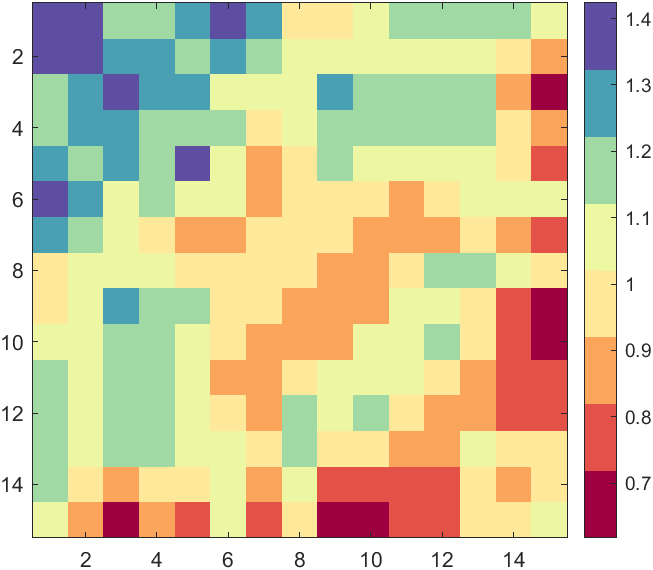
插值
要是自己准备的颜色列表颜色数量少可能会不连续:
XData=rand(15,15);
XData=XData+XData.';
H=fspecial('average',3);
XData=imfilter(XData,H,'replicate');imagesc(XData)
CM=[0.6196    0.0039    0.25880.8874    0.3221    0.28960.9871    0.6459    0.36360.9972    0.9132    0.60340.9300    0.9720    0.63980.6319    0.8515    0.64370.2835    0.6308    0.70080.3686    0.3098    0.6353];
colormap(CM)
colorbar
hold on
ax=gca;
ax.DataAspectRatio=[1,1,1];
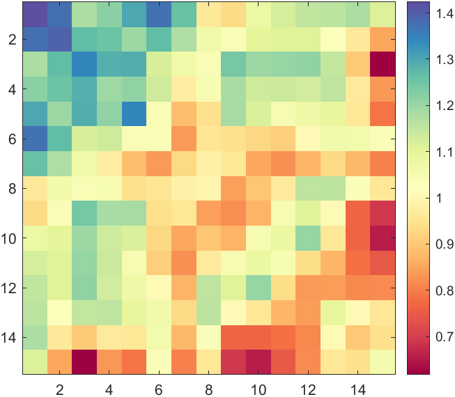
可以对其进行插值:
rng(24)
XData=rand(15,15);
XData=XData+XData.';
H=fspecial('average',3);
XData=imfilter(XData,H,'replicate');imagesc(XData)
CM=[0.6196    0.0039    0.25880.8874    0.3221    0.28960.9871    0.6459    0.36360.9972    0.9132    0.60340.9300    0.9720    0.63980.6319    0.8515    0.64370.2835    0.6308    0.70080.3686    0.3098    0.6353];
CMX=linspace(0,1,size(CM,1));
CMXX=linspace(0,1,256)';
CM=[interp1(CMX,CM(:,1),CMXX,'pchip'),interp1(CMX,CM(:,2),CMXX,'pchip'),interp1(CMX,CM(:,3),CMXX,'pchip')];
colormap(CM)
colorbar
hold on
ax=gca;
ax.DataAspectRatio=[1,1,1];
colormap编辑器
colormapeditor
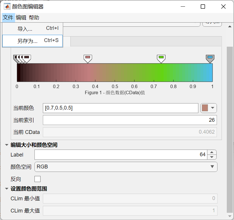
编辑完可以另存工作区,之后存为mat文件:
save CM.mat CustomColormap
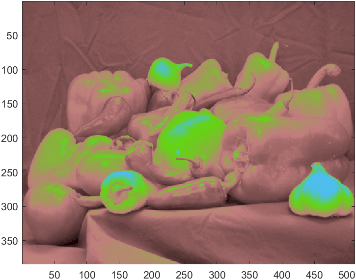
之后画图就可以用啦:
rgbImage=imread("peppers.png");
imagesc(rgb2gray(rgbImage))load CM.mat
colormap(CustomColormap)

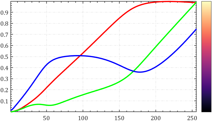
colormap显示
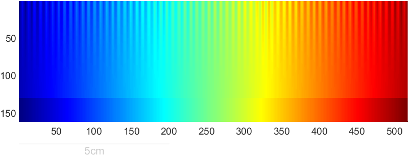
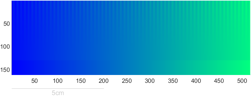
Steve Eddins大佬写了个美观的colormap展示器
Steve Eddins (2023). Colormap Test Image (https://www.mathworks.com/matlabcentral/fileexchange/63726-colormap-test-image), MATLAB Central File Exchange. 检索来源 2023/2/13.
function I = colormapTestImage(map)
% colormapTestImage Create or display colormap test image.
%   I = colormapTestImage creates a grayscale image matrix that is useful
%   for evaluating the effectiveness of colormaps for visualizing
%   sequential data. In particular, the small-amplitude sinusoid pattern at
%   the top of the image is useful for evaluating the perceptual uniformity
%   of a colormap.
%
%   colormapTestImage(map) displays the test image using the specified
%   colormap. The colormap can be specified as the name of a colormap
%   function (such as 'parula' or 'jet'), a function handle to a colormap
%   function (such as @parula or @jet), or a P-by-3 colormap matrix.
%
%   EXAMPLES
%
%     Compute the colormap test image and save it to a file.
%
%       mk = colormapTestImage;
%       imwrite(mk,'test-image.png');
%
%     Compare the perceptual characteristics of the parula and jet
%     colormaps.
%
%       colormapTestImage('parula')
%       colormapTestImage('jet')
%
%   NOTES
%
%   The image is inspired by and adapted from the test image proposed in
%   Peter Kovesi, "Good Colour Maps: How to Design Them," CoRR, 2015,
%   https://arxiv.org/abs/1509.03700
%
%   The upper portion of the image is a linear ramp (from 0.05 to 0.95)
%   with a superimposed sinusoid. The amplitude of the sinusoid ranges from
%   0.05 at the top of the image to 0 at the bottom of the upper portion.
%
%   The lower portion of the image is a pure linear ramp from 0.0 to 1.0.
%
%   This test image differs from Kovesi's in three ways:
%
%     (a) The Kovesi test image superimposes a sinusoid on top of a
%     full-range linear ramp (0 to 1). It then rescales each row
%     independently to have full range, resulting in a linear trend slope
%     that slowly varies from row to row. The modified test image uses the
%     same linear ramp (0.05 to 0.95) on each row, with no need for
%     rescaling.
%
%     (b) The Kovesi test image has exactly 64 sinusoidal cycles
%     horizontally. This test image has 64.5 cycles plus one sample. With
%     this modification, the sinusoid is at the cycle minimum at the left
%     of the image, and it is at the cycle maximum at the right of the
%     image. With this modification, the top row of the modified test image
%     varies from exactly 0.0 on the left to exactly 1.0 on the right,
%     without rescaling.
%
%     (c) The modified test image adds to the bottom of the image a set of
%     rows containing a full-range (0.0 to 1.0) linear ramp with no
%     sinusoidal variation. That makes it easy to view how the colormap
%     appears with a full-range linear ramp.
%
%   Reference: Peter Kovesi, "Good Colour Maps: How to Design Them,"
%   CoRR, 2015, https://arxiv.org/abs/1509.03700%   Steve Eddins
%   Copyright 2017 The MathWorks, Inc.% Compare with 64 in Kovesi 2015. Adding a half-cycle here so that the ramp
% + sinusoid will be at the lowest part of the cycle on the left side of
% the image and at the highest part of the cycle on the right side of the
% image.
num_cycles = 64.5;if nargin < 1I = testImage(num_cycles);
elsedisplayTestImage(map,num_cycles)
endfunction I = testImage(num_cycles)pixels_per_cycle = 8;
A = 0.05;% Compare with width = pixels_per_cycle * num_cycles in Kovesi 2015. Here,
% the extra sample is added to fully reach the peak of the sinusoid on the
% right side of the image.
width = pixels_per_cycle * num_cycles + 1;% Determined by inspection of
% http://peterkovesi.com/projects/colourmaps/colourmaptest.tif
height = round((width - 1) / 4);% The strategy for superimposing a varying-amplitude sinusoid on top of a
% ramp is somewhat different from Kovesi 2015. For each row of the test
% image, Kovesi adds the sinusoid to a full-range ramp and then rescales
% the row so that ramp+sinusoid is full range. A benefit of this approach
% is that each row is full range. A drawback is that the linear trend of
% each row varies as the amplitude of the superimposed sinusoid changes.
%
% Our approach here is a modification. The same linear ramp is used for
% every row of the test image, and it goes from A to 1-A, where A is the
% amplitude of the sinusoid. That way, the linear trend is identical on
% each row. The drawback is that the bottom of the test image goes from
% 0.05 to 0.95 (assuming A = 0.05) instead of from 0.00 to 1.00.
ramp = linspace(A, 1-A, width);k = 0:(width-1);
x = -A*cos((2*pi/pixels_per_cycle) * k);% Amplitude of the superimposed sinusoid varies with the square of the
% distance from the bottom of the image.
q = 0:(height-1);
y = ((height - q) / (height - 1)).^2;
I1 = (y') .* x;% Add the sinusoid to the ramp.
I = I1 + ramp;% Add region to the bottom of the image that is a full-range linear ramp.
I = [I ; repmat(linspace(0,1,width), round(height/4), 1)];function displayTestImage(map,num_cycles)name = '';
if isstring(map)map = char(map);name = map;f = str2func(map);map = f(256);
elseif ischar(map)name = map;f = str2func(map);map = f(256);
elseif isa(map,'function_handle')name = func2str(map);map = map(256);
endI = testImage(num_cycles);
[M,N] = size(I);% Display the image with a width of 2mm per cycle.
display_width_cm = num_cycles * 2 / 10;
display_height_cm = display_width_cm * M / N;fig = figure('Visible','off',...'Color','k');
fig.Units = 'centimeters';% Figure width and height will be image width and height plus 2 cm all the
% way around.
margin = 2;
fig_width = display_width_cm + 2*margin;
fig_height = display_height_cm + 2*margin;
fig.Position(3:4) = [fig_width fig_height];ax = axes('Parent',fig,...'DataAspectRatio',[1 1 1],...'YDir','reverse',...'CLim',[0 1],...'XLim',[0.5 N+0.5],...'YLim',[0.5 M+0.5]);
ax.Units = 'centimeters';
ax.Position = [margin margin display_width_cm display_height_cm];
ax.Units = 'normalized';
box(ax,'off')im = image('Parent',ax,...'CData',I,...'XData',[1 N],...'YData',[1 M],...'CDataMapping','scaled');if ~isempty(name)title(ax,name,'Color',[0.8 0.8 0.8],'Interpreter','none')
end% Draw scale line.
pixels_per_centimeter = N / (display_width_cm);
x = [0.5 5*pixels_per_centimeter];
y = (M + 30) * [1 1];
line('Parent',ax,...'XData',x,...'YData',y,...'Color',[0.8 0.8 0.8],...'Clipping','off');
text(ax,mean(x),y(1),'5cm',...'VerticalAlignment','top',...'HorizontalAlignment','center',...'Color',[0.8 0.8 0.8]);colormap(fig,map)fig.Visible = 'on';
用的时候就正常后面放颜色列表就行:
colormapTestImage(jet)
有趣实例
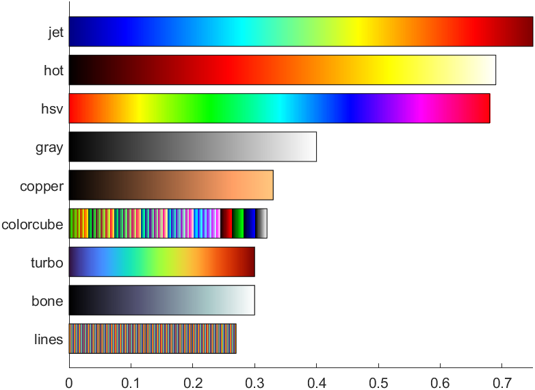
Ned Gulley大佬在迷你黑客大赛有趣的数据分析中给出的图片,展示了各种colormap使用频率排行:
https://blogs.mathworks.com/community/2022/11/08/minihack2022/?s_tid=srchtitle_minihack_1&from=cn
没提供完整代码我自己写了个:
cmaps={'jet','hot','hsv','gray','copper','colorcube','turbo','bone','lines'};
props=[.75,.69,.68,.4,.33,.32,.3,.3,.27];ax=gca;hold on
ax.XLim=[0,max(props)];
ax.YLim=[.3,1.3*length(cmaps)+1];
ax.YTick=(1:length(cmaps)).*1.3;
ax.YTickLabel=cmaps;
ax.YDir='reverse';
for i=1:length(cmaps)c=eval(cmaps{i});c=reshape(c,1,size(c,1),3);image([0,props(i)],[i,i].*1.3,c);rectangle('Position',[0 i.*1.3-.5,props(i) 1])
end
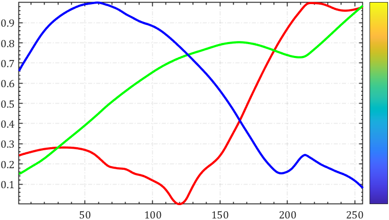
rgbplot
统计colormap中RGB值变化:
rgbplot(parula)
hold on
colormap(parula)
colorbar('Ticks',[])
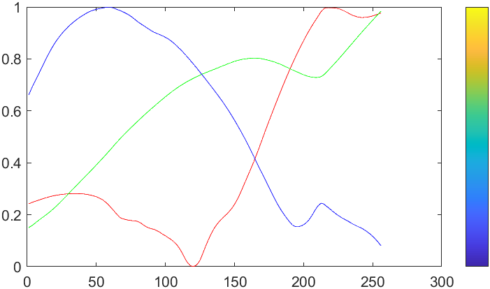
修饰一下能好看点:
rgbplot(parula)
hold on
colormap(parula)
colorbar('Ticks',[])ax=gca;hold on;axis tight
set(ax,'XMinorTick','on','YMinorTick','on','FontName','Cambria',...'XGrid','on','YGrid','on','GridLineStyle','-.','GridAlpha',.1,'LineWidth',.8);
lHdl=findobj(ax,'type','line');
for i=1:length(lHdl)lHdl(i).LineWidth=2;
end
颜色测试图表的识别
需要安装:
Image Processing Toolbox
图像处理工具箱.

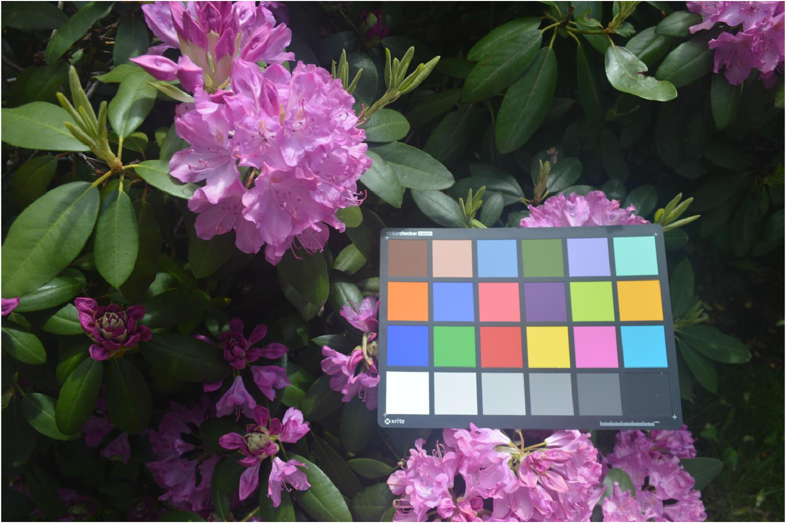
首先展示一下示例图片:
I=imread("colorCheckerTestImage.jpg");
imshow(I)
检测并进行位置标注:
chart=colorChecker(I);
displayChart(chart)
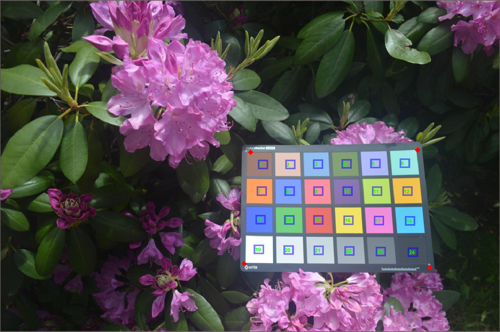
四个角点位置:
chart.RegistrationPoints
ans =
1.0e+03 *
1.3266 0.8282
0.7527 0.8147
0.7734 0.4700
1.2890 0.4632
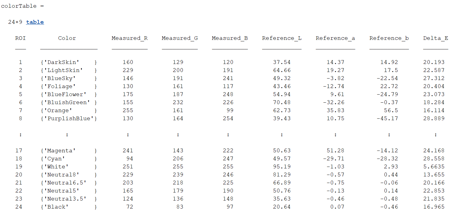
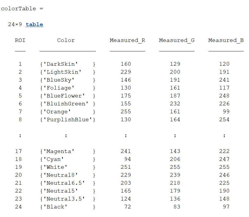
展示检测颜色:
colorTable=measureColor(chart)
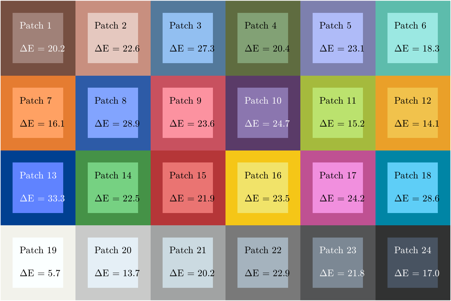
展示标准颜色和检测颜色差别:
figure
displayColorPatch(colorTable)
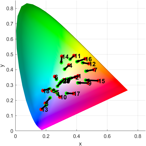
绘制CIE 1976 L* a* b*颜色空间中的测量和参考颜色对比:
figure
plotChromaticity(colorTable)
相关文章:
MATLAB | 有关数值矩阵、颜色图及颜色列表的技巧整理
这是一篇有关数值矩阵、颜色矩阵、颜色列表的技巧整合,会以随笔的形式想到哪写到哪,可能思绪会比较飘逸请大家见谅,本文大体分为以下几个部分: 数值矩阵用颜色显示从颜色矩阵提取颜色从颜色矩阵中提取数据颜色列表相关函数颜色测…...
)
C++模板元编程详细教程(之九)
前序文章请看: C模板元编程详细教程(之一) C模板元编程详细教程(之二) C模板元编程详细教程(之三) C模板元编程详细教程(之四) C模板元编程详细教程(之五&…...
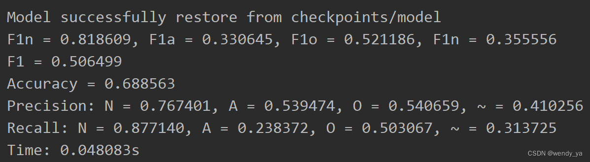
PhysioNet2017分类的代码实现
PhysioNet2017数据集介绍可参考文章:https://wendy.blog.csdn.net/article/details/128686196。本文主要介绍利用PhysioNet2017数据集对其进行分类的代码实现。 目录一、数据集预处理二、训练2.1 导入数据集并进行数据裁剪2.2 划分训练集、验证集和测试集2.3 设置训…...

正大期货本周财经大事抢先看
美国1月CPI、Fed 等央行官员谈话 美国1月超强劲的非农就业人口,让投资人开始上修对这波升息循环利率顶点的预测,也使本周二 (14 日) 的美国 1月 CPI 格外受关注。 介绍正大国际期货主账户对比国内期货的优势 第一点:权限都在主账户 例如…...

html+css综合练习一
文章目录一、小米注册页面1、要求2、案例图3、实现效果3.1、index.html3.2、style.css二、下午茶页面1、要求2、案例图3、index.html4、style.css三、法国巴黎页面1、要求2、案例图3、index.html4、style.css一、小米注册页面 1、要求 阅读下列说明、效果图,进行静…...
安装jdk8
目录标题一、下载地址(一)Linux下载(二)Win下载二、安装(一)Linux(二)Win三、卸载(一)Linux(二)Win一、下载地址 jdk8最新版 jdk8其他…...

二分法心得
原教程见labuladong 首先,我们建议左右区间全部用闭区间。那么第一个搜索区间:left0; rightlen-1; 进入while循环,结束条件是right<left。 然后求mid,如果nums[mid]的值比target大,说明target在左边,…...

Linux安装Docker完整教程
背景最近接手了几个项目,发现项目的部署基本上都是基于Docker的,幸亏在几年前已经熟悉的Docker的基本使用,没有抓瞎。这两年随着云原生的发展,Docker在云原生中的作用使得它也蓬勃发展起来。今天这篇文章就带大家一起实现一下在Li…...

备份基础知识
备份策略可包括:– 整个数据库(整个)– 部分数据库(部分)• 备份类型可指示包含以下项:– 所选文件中的所有数据块(完全备份)– 只限自以前某次备份以来更改过的信息(增量…...

C++学习记录——팔 内存管理
文章目录1、动态内存管理2、内存管理方式operator new operator delete3、new和delete的实现原理1、动态内存管理 C兼容C语言关于内存分配的语法,而添加了C独有的东西。 //int* p1 (int*)malloc(sizeof(int));int* p1 new int;new是一个操作符,C不再需…...

Spring事务失效原因分析解决
文章目录1、方法内部调用2、修饰符3、非运行时异常4、try…catch捕获异常5、多线程调用6、同时使用Transactional和Async7、错误使用事务传播行为8、使用的数据库不支持事务9、是否开启事务支持在工作中,经常会碰到一些事务失效的坑,基于遇到的情况&…...
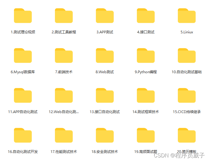
4个月的测试经验,来面试就开口要17K,面试完,我连5K都不想给他.....
2021年8月份我入职了深圳某家创业公司,刚入职还是很兴奋的,到公司一看我傻了,公司除了我一个测试,公司的开发人员就只有3个前端2个后端还有2个UI,在粗略了解公司的业务后才发现是一个从零开始的项目,目前啥…...
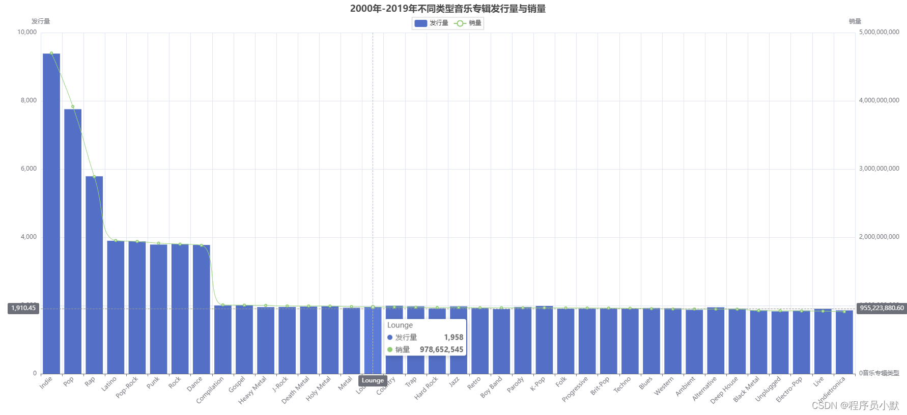
python学习之pyecharts库的使用总结
pyecharts官方文档:https://pyecharts.org//#/zh-cn/ 【1】Timeline 其是一个时间轴组件,如下图红框所示,当点击红色箭头指向的“播放”按钮时,会呈现动画形式展示每一年的数据变化。 data格式为DataFrame,数据如下图…...
【taichi】利用 taichi 编写深度学习算子 —— 以提取右上三角阵为例
本文以取 (bs, n, n) 张量的右上三角阵并展平为向量 (bs, n*(n1)//2)) 为例,展示如何用 taichi 编写深度学习算子。 如图,要把形状为 (bs,n,n)(bs,n,n)(bs,n,n) 的张量,转化为 (bs,n(n1)2)(bs,\frac{n(n1)}{2})(bs,2n(n1)) 的向量。我们先写…...

二进制 k8s 集群下线 worker 组件流程分析和实践
文章目录[toc]事出因果个人思路准备实践当前 worker 节点信息将节点标记为不可调度驱逐节点 pod将 worker 节点从 k8s 集群踢出下线 worker 节点相关组件事出因果 因为之前写了一篇 二进制 k8s 集群下线 master 组件流程分析和实践,所以索性再写一个 worker 节点的缩…...

Bean的六种作用域
限定程序中变量的可用范围叫做作用域,Bean对象的作用域是指Bean对象在Spring整个框架中的某种行为模式~~ Bean对象的六种作用域: singleton:单例作用域(默认) prototype:原型作用域(多例作用域…...

Http发展历史
1 缘起 有一次,听到有人在议论招聘面试的人员, 谈及应聘人员的知识深度,说:问了一些关于Http的问题,如Http相关结构、网络结构等, 然后又说,问没问相关原理、来源? 我也是有些困惑了…...

高级Java程序员必备的技术点,你会了吗?
很多程序员在入行之后的前一两年,快速学习到了做项目常用的各种技术之后,便进入了技术很难寸进的平台期。反正手里掌握的一些技术对于应付普通项目来说,足够用了。因此也会缺入停滞,最终随着年龄的增长,竞争力不断下降…...

【暴力量化】查找最优均线
搜索逻辑 代码主要以支撑概率和压力概率来判断均线的优劣 判断为压力: 当日线与测试均线发生金叉或即将发生金叉后继续下行 判断为支撑: 当日线与测试均线发生死叉或即将发生死叉后继续上行 判断结果的天数: 小于6日均线,用金叉或…...
Java读取mysql导入的文件时中文字段出现�??的乱码如何解决
今天在写程序时遇到了一个乱码问题,困扰了好久,事情是这样的, 在Mapper层编写了查询语句,然后服务处调用,结果控制器返回一堆乱码 然后查看数据源头处: 由重新更改解码的字符集,在数据库中是正…...

什么是IPv6改造
在互联网高速发展的今天,我们日常上网、使用APP、访问网站,背后都离不开IP地址的支撑——IP地址就像是互联网世界的“门牌号”,每一台联网设备、每一个网络节点,都需要一个唯一的IP地址才能实现互联互通。随着物联网、5G、云计算、…...

AI翻译测试案例:多语言文档错误预防秘籍
在全球化软件开发生态中,多语言支持已成为标配功能,但随之而来的翻译错误却可能引发用户体验灾难——从文化误解到功能失效。作为软件测试从业者,您深知测试案例是质量保障的核心工具,而AI翻译技术的崛起正为多语言文档测试带来革…...

Qwen3在软件测试中的应用:自动生成测试用例视觉报告
Qwen3在软件测试中的应用:自动生成测试用例视觉报告 你是不是也经历过这样的场景?测试过程中发现了一个bug,费了九牛二虎之力复现、定位,最后却卡在了写报告上。截图、录屏、整理日志、描述步骤、分析根因……一套流程下来&#…...

STM32F042 CAN调试实战:从端口映射到波形捕获的完整指南
1. STM32F042 CAN调试入门指南 第一次接触STM32F042的CAN总线调试时,我也遇到了不少坑。这个SSOP20封装的芯片引脚资源有限,PA11和PA12默认并不是CAN功能引脚,需要进行端口映射。很多新手在这里就会踩坑,直接使用SYSCFG_MemoryRem…...

ServiceAccount 与 RBAC 的关系
什么是 ServiceAccount 与精细化的 RBAC 策略在 Kubernetes 里,很多人一开始会把注意力放在 Pod、Deployment、Service 这些资源上,觉得把应用跑起来就差不多了。可问题是,应用跑起来之后,如果它要去访问 Kubernetes API 呢&#…...

HI3516DV300的SDIO1接口实战:RTL8822BS WiFi模块移植避坑指南
HI3516DV300的SDIO1接口实战:RTL8822BS WiFi模块移植避坑指南 在嵌入式系统开发中,WiFi模块的集成往往是项目成功的关键因素之一。海思HI3516DV300作为一款广泛应用于智能摄像头领域的SoC,其SDIO1接口与RTL8822BS WiFi模块的配合使用…...

Spring AOP避坑指南:如何用@Around实现完美的日志与事务管理
Spring AOP高阶实战:Around在日志与事务中的精妙运用 1. 为什么Around是AOP中的瑞士军刀 在Spring生态中,AOP(面向切面编程)就像是一位隐形的助手,默默处理着那些横切关注点。而Around通知,无疑是这位助手手…...

业余无线电B类考试高效复习指南:四轮刷题法与核心知识点速记
1. 四轮刷题法:从700题到200题的高效路径 第一次接触业余无线电B类考试题库时,700多道题目确实会让人望而生畏。但别担心,这套经过实战检验的四轮刷题法,能帮你把复习量压缩70%以上。我当年备考时就用这个方法,最终只重…...

无人机与手机照片POS信息提取工具|支持JPG批量读取与导出
温馨提示:文末有联系方式工具核心功能概述 本工具专为地理信息与航测工作者设计,可高效提取无人机航拍影像及普通智能手机拍摄的JPG照片中嵌入的POS(Position and Orientation System)元数据,涵盖经度、纬度、海拔、拍…...

KingbaseES集群运维案例之--主备发生故障,主库能正常使用,备库无法启用
KingbaseES集群运维案例之–主备发生故障,主库能正常使用,备库无法启用 案例:主备发生故障,主库能正常使用,备库无法启用 文章目录KingbaseES集群运维案例之--主备发生故障,主库能正常使用,备库…...