Retinanet网络与focal loss损失
参考代码:https://github.com/yhenon/pytorch-retinanet
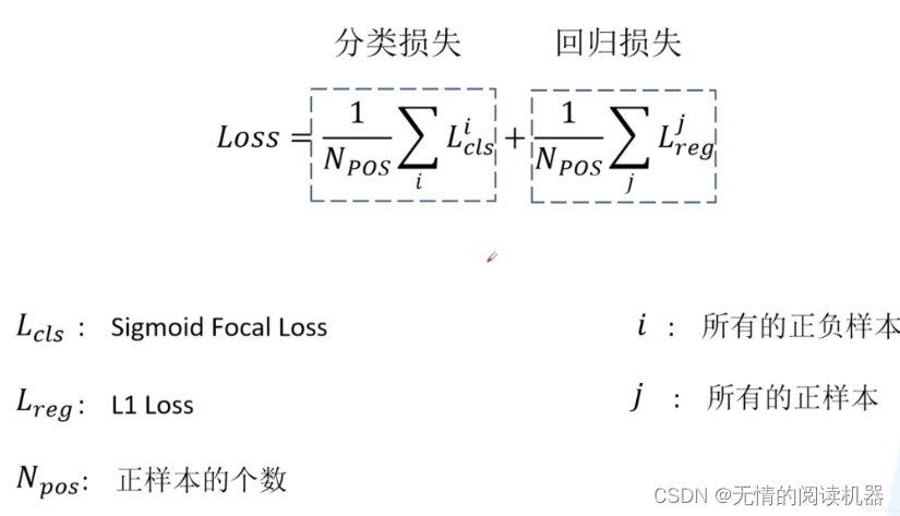
1.损失函数
1)原理
本文一个核心的贡献点就是 focal loss。总损失依然分为两部分,一部分是分类损失,一部分是回归损失。
在讲分类损失之前,我们来回顾一下二分类交叉熵损失 (binary_cross_entropy)。
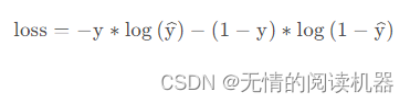
计算代码如下:
import numpy as npy_true = np.array([0., 1., 1., 1., 1., 1., 1., 1., 1., 1.])
y_pred = np.array([0.2, 0.8, 0.8, 0.8, 0.8, 0.8, 0.8, 0.8, 0.8, 0.8])my_loss = - y_true * np.log(y_pred) - (1 - y_true) * np.log(1 - y_pred)
mean_my_loss = np.mean(my_loss)
print("mean_my_loss:",mean_my_loss)![]()
调用pytorch自带的函数计算
import torch.nn.functional as F
import numpy as np
import torch
torch_pred = torch.tensor(y_pred)
torch_true = torch.tensor(y_true)
bce_loss = F.binary_cross_entropy(torch_pred, torch_true)
print('bce_loss:', bce_loss)

现在回到focal loss,Focal loss的起源是二分类交叉熵。
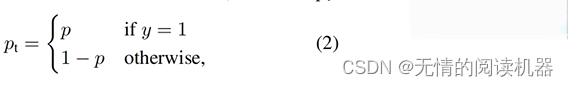
二分类的交叉熵损失还可以如下表示,其中y∈{1,-1},1代表候选框是正样本,-1代表是负样本:

为了表示方便,可以定义如下公式:
那么问题来了,应用场景如下:
在one-stage 物体检测模型中,一张图中能匹配到目标的候选框(正样本)大概是十几个到几十个,然后没有匹配到的候选框(负样本)10 的四次方到五次方。这些负样本中,大部分都是简单易分的样本,对于训练样本起不到作用,反而淹没了有助于训练的样本。
举个例子,正样本有50个,损失是3,负样本是10000个,损失是0.1
那么50x3 = 150,10000x0.1=1000

所以,为了平衡交叉熵,采用了系数αt,当是正样本的时候,αt = α,负样本的时候 αt=1-α,α∈[0,1]
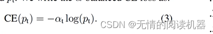
αt能平衡正负样本的权重,但是不能区分哪些是困难样本,哪些是容易样本(是否对训练有帮助)。
所以继续引入公式,这样就解决了区分样本容易性的问题:

最后,结合两个公式,形成最终的公式。

展开形式如下
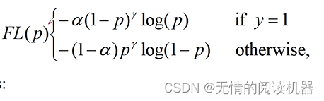
现在来看一下效果,p代表预测候选框是正样本的概率,y是候选框实际上是正样本还是负样本,CE是普通交叉熵计算的损失,FL是focal loss,rate是缩小的比例。可以看出,最后两行难区分样本的rate很小。

2)代码
import numpy as np
import torch
import torch.nn as nnclass FocalLoss(nn.Module):#def __init__(self):def forward(self, classifications, regressions, anchors, annotations):alpha = 0.25gamma = 2.0# classifications是预测结果batch_size = classifications.shape[0]# 分类lossclassification_losses = []# 回归lossregression_losses = []# anchors的形状是 [1, 每层anchor数量之和 , 4]anchor = anchors[0, :, :]anchor_widths  = anchor[:, 2] - anchor[:, 0]  # x2-x1anchor_heights = anchor[:, 3] - anchor[:, 1]  # y2-y1anchor_ctr_x   = anchor[:, 0] + 0.5 * anchor_widths  # 中心点x坐标anchor_ctr_y   = anchor[:, 1] + 0.5 * anchor_heights  # 中心点y坐标for j in range(batch_size):# classifications的shape [batch,所有anchor的数量,分类数]classification = classifications[j, :, :]# classifications的shape [batch,所有anchor的数量,分类数]regression = regressions[j, :, :]bbox_annotation = annotations[j, :, :]bbox_annotation = bbox_annotation[bbox_annotation[:, 4] != -1]classification = torch.clamp(classification, 1e-4, 1.0 - 1e-4)if bbox_annotation.shape[0] == 0:if torch.cuda.is_available():alpha_factor = torch.ones(classification.shape).cuda() * alphaalpha_factor = 1. - alpha_factorfocal_weight = classificationfocal_weight = alpha_factor * torch.pow(focal_weight, gamma)bce = -(torch.log(1.0 - classification))# cls_loss = focal_weight * torch.pow(bce, gamma)cls_loss = focal_weight * bceclassification_losses.append(cls_loss.sum())regression_losses.append(torch.tensor(0).float().cuda())else:alpha_factor = torch.ones(classification.shape) * alphaalpha_factor = 1. - alpha_factorfocal_weight = classificationfocal_weight = alpha_factor * torch.pow(focal_weight, gamma)bce = -(torch.log(1.0 - classification))# cls_loss = focal_weight * torch.pow(bce, gamma)cls_loss = focal_weight * bceclassification_losses.append(cls_loss.sum())regression_losses.append(torch.tensor(0).float())continue# 每个anchor 与 每个标注的真实框的iouIoU = calc_iou(anchors[0, :, :], bbox_annotation[:, :4]) # num_anchors x num_annotations# 每个anchor对应的最大的iou (anchor与grandtruce进行配对)# 得到了配对的索引和对应的最大值IoU_max, IoU_argmax = torch.max(IoU, dim=1)#import pdb#pdb.set_trace()# compute the loss for classification# classification 的shape[anchor总数,分类数]targets = torch.ones(classification.shape) * -1if torch.cuda.is_available():targets = targets.cuda()# 判断每个元素是否小于0.4 小于就返回true(anchor对应的最大iou<0.4,那就是背景)targets[torch.lt(IoU_max, 0.4), :] = 0# 最大iou大于0.5的anchor索引positive_indices = torch.ge(IoU_max, 0.5)num_positive_anchors = positive_indices.sum()assigned_annotations = bbox_annotation[IoU_argmax, :]targets[positive_indices, :] = 0targets[positive_indices, assigned_annotations[positive_indices, 4].long()] = 1if torch.cuda.is_available():alpha_factor = torch.ones(targets.shape).cuda() * alphaelse:alpha_factor = torch.ones(targets.shape) * alphaalpha_factor = torch.where(torch.eq(targets, 1.), alpha_factor, 1. - alpha_factor)focal_weight = torch.where(torch.eq(targets, 1.), 1. - classification, classification)focal_weight = alpha_factor * torch.pow(focal_weight, gamma)bce = -(targets * torch.log(classification) + (1.0 - targets) * torch.log(1.0 - classification))# cls_loss = focal_weight * torch.pow(bce, gamma)cls_loss = focal_weight * bceif torch.cuda.is_available():cls_loss = torch.where(torch.ne(targets, -1.0), cls_loss, torch.zeros(cls_loss.shape).cuda())else:cls_loss = torch.where(torch.ne(targets, -1.0), cls_loss, torch.zeros(cls_loss.shape))classification_losses.append(cls_loss.sum()/torch.clamp(num_positive_anchors.float(), min=1.0))# compute the loss for regressionif positive_indices.sum() > 0:assigned_annotations = assigned_annotations[positive_indices, :]anchor_widths_pi = anchor_widths[positive_indices]anchor_heights_pi = anchor_heights[positive_indices]anchor_ctr_x_pi = anchor_ctr_x[positive_indices]anchor_ctr_y_pi = anchor_ctr_y[positive_indices]gt_widths  = assigned_annotations[:, 2] - assigned_annotations[:, 0]gt_heights = assigned_annotations[:, 3] - assigned_annotations[:, 1]gt_ctr_x   = assigned_annotations[:, 0] + 0.5 * gt_widthsgt_ctr_y   = assigned_annotations[:, 1] + 0.5 * gt_heights# clip widths to 1gt_widths  = torch.clamp(gt_widths, min=1)gt_heights = torch.clamp(gt_heights, min=1)targets_dx = (gt_ctr_x - anchor_ctr_x_pi) / anchor_widths_pitargets_dy = (gt_ctr_y - anchor_ctr_y_pi) / anchor_heights_pitargets_dw = torch.log(gt_widths / anchor_widths_pi)targets_dh = torch.log(gt_heights / anchor_heights_pi)targets = torch.stack((targets_dx, targets_dy, targets_dw, targets_dh))targets = targets.t()if torch.cuda.is_available():targets = targets/torch.Tensor([[0.1, 0.1, 0.2, 0.2]]).cuda()else:targets = targets/torch.Tensor([[0.1, 0.1, 0.2, 0.2]])negative_indices = 1 + (~positive_indices)regression_diff = torch.abs(targets - regression[positive_indices, :])regression_loss = torch.where(torch.le(regression_diff, 1.0 / 9.0),0.5 * 9.0 * torch.pow(regression_diff, 2),regression_diff - 0.5 / 9.0)regression_losses.append(regression_loss.mean())else:if torch.cuda.is_available():regression_losses.append(torch.tensor(0).float().cuda())else:regression_losses.append(torch.tensor(0).float())return torch.stack(classification_losses).mean(dim=0, keepdim=True), torch.stack(regression_losses).mean(dim=0, keepdim=True)
3)分类损失的计算过程
假设一张图片有n个anchor,有m个grandtrue,有L个类别
1.得到anchor和每一个grandtrue的IOU
# 每个anchor 与 每个标注的真实框的iou
IoU = calc_iou(anchors[0, :, :], bbox_annotation[:, :4]) # num_anchors x num_annotations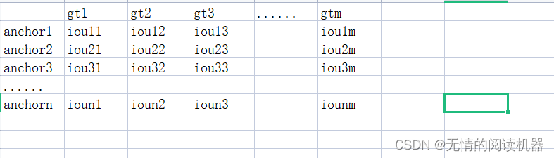
2.得到每个anchor最大的IOU,以及对应的grandtrue
IoU_max, IoU_argmax = torch.max(IoU, dim=1)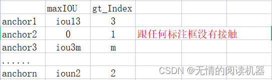
3.初始化一个分类目标结果表,默认值是-1
targets = torch.ones(classification.shape) * -1 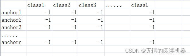
4.如果某个anchor的最大IOU<0.4,那么它对应的分类全为0
targets[torch.lt(IoU_max, 0.4), :] = 0例如:iou3m = 0.3,ioun2 = 0.2
此时,上述分类结果表就更新anchor3,和anchorn的分类结果

5.把每个anchor关联对应的grandtruce信息,其中参数5是预测的类别
# 最大iou大于0.5的anchor索引
positive_indices = torch.ge(IoU_max, 0.5)num_positive_anchors = positive_indices.sum()assigned_annotations = bbox_annotation[IoU_argmax, :]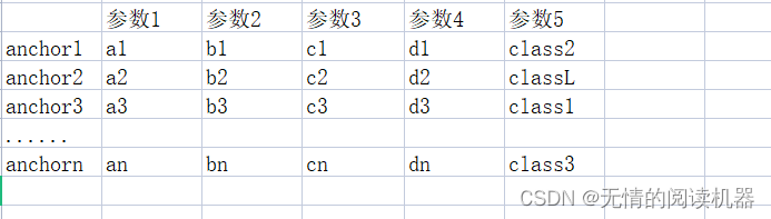 6.如果anchor的最大IOU>0.5,那么根据参数5,修改对应的分类结果表为one-hot形式
targets[positive_indices, :] = 0
targets[positive_indices, assigned_annotations[positive_indices, 4].long()] = 1
例如 iou12 = 0.6,参数5 = class2
修改分类结果表
7. 得到损失的权重部分
alpha_factor = torch.where(torch.eq(targets, 1.), alpha_factor, 1. - alpha_factor)
focal_weight = torch.where(torch.eq(targets, 1.), 1. - classification, classification)
focal_weight = alpha_factor * torch.pow(focal_weight, gamma)
α表,将0的地方替换成1-α,1的地方替换成 α

p表 将0的地方原概率,1的地方换成1-p

权重表的元素就是两表对应元素的乘积
8.得到损失的损失部分
bce = -(targets * torch.log(classification) + (1.0 - targets) * torch.log(1.0 - classification))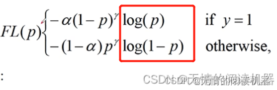
9.得到初步的损失结果
cls_loss = focal_weight * bce10.将分类结果表原本是-1的地方,对应的损失变成0
例如anchor2最大iou是0.45,介于0.4与0.5之间,我们就不计算他的损失,忽略不计
if torch.cuda.is_available():cls_loss = torch.where(torch.ne(targets, -1.0), cls_loss, torch.zeros(cls_loss.shape).cuda())
else:cls_loss = torch.where(torch.ne(targets, -1.0), cls_loss, torch.zeros(cls_loss.shape))
11.损失汇总
classification_losses.append(cls_loss.sum()/torch.clamp(num_positive_anchors.float(), min=1.0))2.网络结构
整体来讲,网络采用了FPN模型
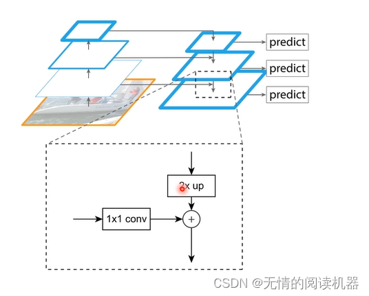
 这个结构也是可以变的(可以灵活改变),如下所示

模型如下所示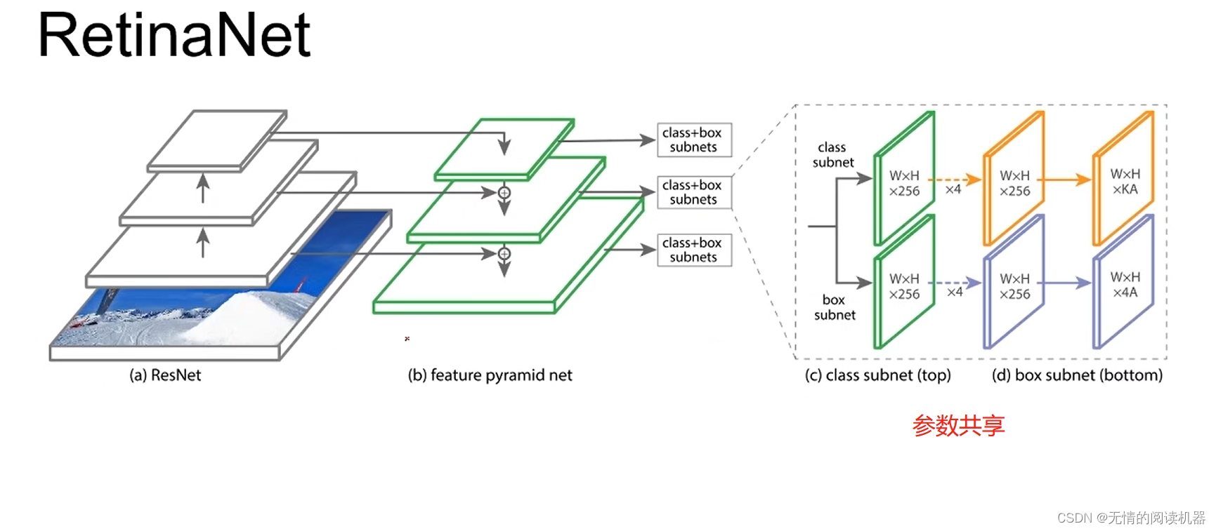
其中每个位置的anchor是9个,三个形状x三个比例
K是分类的数量,A是每个位置anchor是数量
4A,4是四个参数可以确定anchor的位置和大小。
3.代码讲解:
1.FPN分支部分
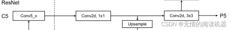
self.P5_1 = nn.Conv2d(C5_size, feature_size, kernel_size=1, stride=1, padding=0)
self.P5_upsampled = nn.Upsample(scale_factor=2, mode='nearest')
self.P5_2 = nn.Conv2d(feature_size, feature_size, kernel_size=3, stride=1, padding=1)
self.P4_1 = nn.Conv2d(C4_size, feature_size, kernel_size=1, stride=1, padding=0)
self.P4_upsampled = nn.Upsample(scale_factor=2, mode='nearest')
self.P4_2 = nn.Conv2d(feature_size, feature_size, kernel_size=3, stride=1, padding=1)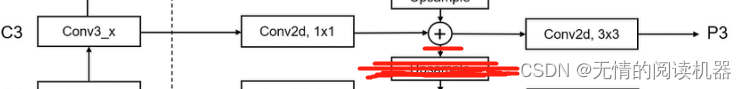
self.P3_1 = nn.Conv2d(C3_size, feature_size, kernel_size=1, stride=1, padding=0)
self.P3_2 = nn.Conv2d(feature_size, feature_size, kernel_size=3, stride=1, padding=1) 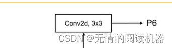
self.P6 = nn.Conv2d(C5_size, feature_size, kernel_size=3, stride=2, padding=1) 
self.P7_1 = nn.ReLU()
self.P7_2 = nn.Conv2d(feature_size, feature_size, kernel_size=3, stride=2, padding=1)
forward
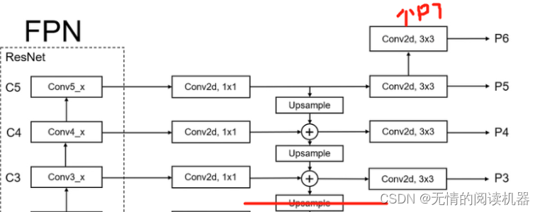
def forward(self, inputs):#inputs 是主干模块conv3、conv4、conv5的输出C3, C4, C5 = inputsP5_x = self.P5_1(C5)P5_upsampled_x = self.P5_upsampled(P5_x)P5_x = self.P5_2(P5_x)P4_x = self.P4_1(C4)P4_x = P5_upsampled_x + P4_xP4_upsampled_x = self.P4_upsampled(P4_x)P4_x = self.P4_2(P4_x)P3_x = self.P3_1(C3)P3_x = P3_x + P4_upsampled_xP3_x = self.P3_2(P3_x)P6_x = self.P6(C5)P7_x = self.P7_1(P6_x)P7_x = self.P7_2(P7_x)return [P3_x, P4_x, P5_x, P6_x, P7_x]
2.回归自网络

class RegressionModel(nn.Module):def __init__(self, num_features_in, num_anchors=9, feature_size=256):super(RegressionModel, self).__init__()#其实num_features_in就等于256self.conv1 = nn.Conv2d(num_features_in, feature_size, kernel_size=3, padding=1)self.act1 = nn.ReLU()self.conv2 = nn.Conv2d(feature_size, feature_size, kernel_size=3, padding=1)self.act2 = nn.ReLU()self.conv3 = nn.Conv2d(feature_size, feature_size, kernel_size=3, padding=1)self.act3 = nn.ReLU()self.conv4 = nn.Conv2d(feature_size, feature_size, kernel_size=3, padding=1)self.act4 = nn.ReLU()#4个参数就能确定anchor的大小self.output = nn.Conv2d(feature_size, num_anchors * 4, kernel_size=3, padding=1)def forward(self, x):out = self.conv1(x)out = self.act1(out)out = self.conv2(out)out = self.act2(out)out = self.conv3(out)out = self.act3(out)out = self.conv4(out)out = self.act4(out)out = self.output(out)# out is B x C x W x H, with C = 4*num_anchorsout = out.permute(0, 2, 3, 1)#相当于展平了,-1的位置相当于所有anchor的数目return out.contiguous().view(out.shape[0], -1, 4)3.分类网络

class ClassificationModel(nn.Module):def __init__(self, num_features_in, num_anchors=9, num_classes=80, prior=0.01, feature_size=256):super(ClassificationModel, self).__init__()self.num_classes = num_classesself.num_anchors = num_anchorsself.conv1 = nn.Conv2d(num_features_in, feature_size, kernel_size=3, padding=1)self.act1 = nn.ReLU()self.conv2 = nn.Conv2d(feature_size, feature_size, kernel_size=3, padding=1)self.act2 = nn.ReLU()self.conv3 = nn.Conv2d(feature_size, feature_size, kernel_size=3, padding=1)self.act3 = nn.ReLU()self.conv4 = nn.Conv2d(feature_size, feature_size, kernel_size=3, padding=1)self.act4 = nn.ReLU()self.output = nn.Conv2d(feature_size, num_anchors * num_classes, kernel_size=3, padding=1)self.output_act = nn.Sigmoid()def forward(self, x):out = self.conv1(x)out = self.act1(out)out = self.conv2(out)out = self.act2(out)out = self.conv3(out)out = self.act3(out)out = self.conv4(out)out = self.act4(out)out = self.output(out)out = self.output_act(out)# out is B x C x W x H, with C = n_classes + n_anchorsout1 = out.permute(0, 2, 3, 1)batch_size, width, height, channels = out1.shapeout2 = out1.view(batch_size, width, height, self.num_anchors, self.num_classes)return out2.contiguous().view(x.shape[0], -1, self.num_classes)4.主干网络、训练和预测过程
1.网络结构

经过conv1缩小4倍,经过conv2不变,conv3、v4,v5都缩小两倍,p5到p6缩小两倍,p6到p7缩小两倍
p3相对于图片缩小了2的3次方,p4相对于图片缩小了2的4次方,以此类推
class ResNet(nn.Module):#layers是层数def __init__(self, num_classes, block, layers):self.inplanes = 64super(ResNet, self).__init__()#这个是输入 conv1self.conv1 = nn.Conv2d(3, 64, kernel_size=7, stride=2, padding=3, bias=False)self.bn1 = nn.BatchNorm2d(64)self.relu = nn.ReLU(inplace=True)self.maxpool = nn.MaxPool2d(kernel_size=3, stride=2, padding=1)#这是c2self.layer1 = self._make_layer(block, 64, layers[0])#这是c3self.layer2 = self._make_layer(block, 128, layers[1], stride=2)#这是c4self.layer3 = self._make_layer(block, 256, layers[2], stride=2)#这是c5self.layer4 = self._make_layer(block, 512, layers[3], stride=2)#得到c3、c4、c5输出的通道数if block == BasicBlock:fpn_sizes = [self.layer2[layers[1] - 1].conv2.out_channels, self.layer3[layers[2] - 1].conv2.out_channels,self.layer4[layers[3] - 1].conv2.out_channels]elif block == Bottleneck:fpn_sizes = [self.layer2[layers[1] - 1].conv3.out_channels, self.layer3[layers[2] - 1].conv3.out_channels,self.layer4[layers[3] - 1].conv3.out_channels]else:raise ValueError(f"Block type {block} not understood")#创建FPN的分支部分self.fpn = PyramidFeatures(fpn_sizes[0], fpn_sizes[1], fpn_sizes[2])#创建回归网络self.regressionModel = RegressionModel(256)#创建分类网络self.classificationModel = ClassificationModel(256, num_classes=num_classes)self.anchors = Anchors()self.regressBoxes = BBoxTransform()self.clipBoxes = ClipBoxes()self.focalLoss = losses.FocalLoss()#权重初始化for m in self.modules():if isinstance(m, nn.Conv2d):n = m.kernel_size[0] * m.kernel_size[1] * m.out_channelsm.weight.data.normal_(0, math.sqrt(2. / n))elif isinstance(m, nn.BatchNorm2d):m.weight.data.fill_(1)m.bias.data.zero_()prior = 0.01self.classificationModel.output.weight.data.fill_(0)self.classificationModel.output.bias.data.fill_(-math.log((1.0 - prior) / prior))self.regressionModel.output.weight.data.fill_(0)self.regressionModel.output.bias.data.fill_(0)#冻结bn层参数更新,因为预训练的参数已经很好了self.freeze_bn()def _make_layer(self, block, planes, blocks, stride=1):downsample = Noneif stride != 1 or self.inplanes != planes * block.expansion:downsample = nn.Sequential(nn.Conv2d(self.inplanes, planes * block.expansion,kernel_size=1, stride=stride, bias=False),nn.BatchNorm2d(planes * block.expansion),)layers = [block(self.inplanes, planes, stride, downsample)]self.inplanes = planes * block.expansionfor i in range(1, blocks):layers.append(block(self.inplanes, planes))return nn.Sequential(*layers)def freeze_bn(self):'''Freeze BatchNorm layers.'''for layer in self.modules():if isinstance(layer, nn.BatchNorm2d):layer.eval()2.训练过程和预测过程
1)anchor的调整
生成的预测值 regression [batch, anchor的数量,4] regression[:, :, 0]和[:, :, 1]用来移动anchor中心点 [:, :, 2]和[:, :, 3]用来改变框子的长度
import torch.nn as nn
import torch
import numpy as np# 生成的预测值 regression [batch, anchor的数量,4]  regression[:, :, 0]和[:, :, 1]用来移动anchor中心点 [:, :, 2]和[:, :, 3]用来改变框子的长度
class BBoxTransform(nn.Module):def __init__(self, mean=None, std=None):super(BBoxTransform, self).__init__()if mean is None:if torch.cuda.is_available():self.mean = torch.from_numpy(np.array([0, 0, 0, 0]).astype(np.float32)).cuda()else:self.mean = torch.from_numpy(np.array([0, 0, 0, 0]).astype(np.float32))else:self.mean = meanif std is None:if torch.cuda.is_available():self.std = torch.from_numpy(np.array([0.1, 0.1, 0.2, 0.2]).astype(np.float32)).cuda()else:self.std = torch.from_numpy(np.array([0.1, 0.1, 0.2, 0.2]).astype(np.float32))else:self.std = stddef forward(self, boxes, deltas):#boxes就是图片所有的anchor[batch , 一张图片上anchor的总数 ,4]widths  = boxes[:, :, 2] - boxes[:, :, 0]  # x2 - x1 = 宽heights = boxes[:, :, 3] - boxes[:, :, 1]  # y2 - y1 = 高ctr_x   = boxes[:, :, 0] + 0.5 * widths    # x1 + 宽/2 = 中心点 xctr_y   = boxes[:, :, 1] + 0.5 * heights   # y1 + 高/2 = 中心点 ydx = deltas[:, :, 0] * self.std[0] + self.mean[0]dy = deltas[:, :, 1] * self.std[1] + self.mean[1]dw = deltas[:, :, 2] * self.std[2] + self.mean[2]dh = deltas[:, :, 3] * self.std[3] + self.mean[3]pred_ctr_x = ctr_x + dx * widthspred_ctr_y = ctr_y + dy * heightspred_w     = torch.exp(dw) * widthspred_h     = torch.exp(dh) * heightspred_boxes_x1 = pred_ctr_x - 0.5 * pred_wpred_boxes_y1 = pred_ctr_y - 0.5 * pred_hpred_boxes_x2 = pred_ctr_x + 0.5 * pred_wpred_boxes_y2 = pred_ctr_y + 0.5 * pred_hpred_boxes = torch.stack([pred_boxes_x1, pred_boxes_y1, pred_boxes_x2, pred_boxes_y2], dim=2)return pred_boxes
2总过程
def forward(self, inputs):if self.training:img_batch, annotations = inputselse:img_batch = inputsx = self.conv1(img_batch)x = self.bn1(x)x = self.relu(x)x = self.maxpool(x)x1 = self.layer1(x)x2 = self.layer2(x1)x3 = self.layer3(x2)x4 = self.layer4(x3)features = self.fpn([x2, x3, x4])#shape[batch,每次anchor总数之和,4个值]regression = torch.cat([self.regressionModel(feature) for feature in features], dim=1)# shape[batch,每次anchor总数之和,分类个数]classification = torch.cat([self.classificationModel(feature) for feature in features], dim=1)anchors = self.anchors(img_batch)if self.training:return self.focalLoss(classification, regression, anchors, annotations)else:#得到调节参数之后的框子transformed_anchors = self.regressBoxes(anchors, regression)#保证框子在图片之内transformed_anchors = self.clipBoxes(transformed_anchors, img_batch)finalResult = [[], [], []]#每个框对应类别的置信度finalScores = torch.Tensor([])#框对应的分类序号:第几类finalAnchorBoxesIndexes = torch.Tensor([]).long()#框的坐标finalAnchorBoxesCoordinates = torch.Tensor([])if torch.cuda.is_available():finalScores = finalScores.cuda()finalAnchorBoxesIndexes = finalAnchorBoxesIndexes.cuda()finalAnchorBoxesCoordinates = finalAnchorBoxesCoordinates.cuda()for i in range(classification.shape[2]):scores = torch.squeeze(classification[:, :, i])scores_over_thresh = (scores > 0.05)if scores_over_thresh.sum() == 0:# no boxes to NMS, just continuecontinuescores = scores[scores_over_thresh]anchorBoxes = torch.squeeze(transformed_anchors)anchorBoxes = anchorBoxes[scores_over_thresh]anchors_nms_idx = nms(anchorBoxes, scores, 0.5)finalResult[0].extend(scores[anchors_nms_idx])finalResult[1].extend(torch.tensor([i] * anchors_nms_idx.shape[0]))finalResult[2].extend(anchorBoxes[anchors_nms_idx])finalScores = torch.cat((finalScores, scores[anchors_nms_idx]))finalAnchorBoxesIndexesValue = torch.tensor([i] * anchors_nms_idx.shape[0])if torch.cuda.is_available():finalAnchorBoxesIndexesValue = finalAnchorBoxesIndexesValue.cuda()finalAnchorBoxesIndexes = torch.cat((finalAnchorBoxesIndexes, finalAnchorBoxesIndexesValue))finalAnchorBoxesCoordinates = torch.cat((finalAnchorBoxesCoordinates, anchorBoxes[anchors_nms_idx]))return [finalScores, finalAnchorBoxesIndexes, finalAnchorBoxesCoordinates]5.两种block的定义
import torch.nn as nndef conv3x3(in_planes, out_planes, stride=1):"""3x3 convolution with padding"""return nn.Conv2d(in_planes, out_planes, kernel_size=3, stride=stride,padding=1, bias=False)class BasicBlock(nn.Module):expansion = 1def __init__(self, inplanes, planes, stride=1, downsample=None):super(BasicBlock, self).__init__()self.conv1 = conv3x3(inplanes, planes, stride)self.bn1 = nn.BatchNorm2d(planes)self.relu = nn.ReLU(inplace=True)self.conv2 = conv3x3(planes, planes)self.bn2 = nn.BatchNorm2d(planes)self.downsample = downsampleself.stride = stridedef forward(self, x):residual = xout = self.conv1(x)out = self.bn1(out)out = self.relu(out)out = self.conv2(out)out = self.bn2(out)if self.downsample is not None:residual = self.downsample(x)out += residualout = self.relu(out)return outclass Bottleneck(nn.Module):expansion = 4def __init__(self, inplanes, planes, stride=1, downsample=None):super(Bottleneck, self).__init__()self.conv1 = nn.Conv2d(inplanes, planes, kernel_size=1, bias=False)self.bn1 = nn.BatchNorm2d(planes)self.conv2 = nn.Conv2d(planes, planes, kernel_size=3, stride=stride,padding=1, bias=False)self.bn2 = nn.BatchNorm2d(planes)self.conv3 = nn.Conv2d(planes, planes * 4, kernel_size=1, bias=False)self.bn3 = nn.BatchNorm2d(planes * 4)self.relu = nn.ReLU(inplace=True)self.downsample = downsampleself.stride = stridedef forward(self, x):residual = xout = self.conv1(x)out = self.bn1(out)out = self.relu(out)out = self.conv2(out)out = self.bn2(out)out = self.relu(out)out = self.conv3(out)out = self.bn3(out)if self.downsample is not None:residual = self.downsample(x)out += residualout = self.relu(out)return out6.anchor
1.每个位置的生成anchor函数
anchor的生成都是以原图为基准的这个函数的作用是生成一个位置中所有的anchor,形式是(x1,y1,x2,y2)并且(X1,y1)和(x2,y2)关于中心对称,这样给定一个中点,可以直接拿(x1,y1,x2,y2)计算出相应的anchor
大概功能步骤:
1.确定每个位置anchor的数量:宽高比例数量x边长缩放比例数量
2.得到anchor的标准边长缩放后的结果 :base_size x scales
3.通过上述结果得到标准面积:(base_size x scales)的平方
2.通过h = sqrt(areas / ratio)和w = h * ratio得到宽高
3.得到每个anchor的两个坐标 (0-h/2 , 0-w/2) 和 (h/2 , w/2)
4.输出anchor
def generate_anchors(base_size=16, ratios=None, scales=None):"""Generate anchor (reference) windows by enumerating aspect ratios Xscales w.r.t. a reference window."""if ratios is None:ratios = np.array([0.5, 1, 2])if scales is None:scales = np.array([2 ** 0, 2 ** (1.0 / 3.0), 2 ** (2.0 / 3.0)])#每个位置的anchor总数 n种规模 * m种比例num_anchors = len(ratios) * len(scales)# 初始化anchor的参数 x,y,w,hanchors = np.zeros((num_anchors, 4))# scale base_size#np.tile(scales, (2, len(ratios))).T结果如下:#[[1. 1. ]# [1.25992105 1.25992105]# [1.58740105 1.58740105]# [1. 1. ]# [1.25992105 1.25992105]# [1.58740105 1.58740105]# [1. 1. ]# [1.25992105 1.25992105]# [1.58740105 1.58740105]]# shape (9, 2)#设置anchor的w、h的基础大小(1:1)anchors[:, 2:] = base_size * np.tile(scales, (2, len(ratios))).T# 计算anchor的基础面积#[area1,area2,area3,area1,area2,area3,area1,area2,area3]areas = anchors[:, 2] * anchors[:, 3]# correct for ratios#利用面积和宽高比得到真正的宽和高#根据公式1: areas / (w/h) = areas / ratio = hxh => h = sqrt(areas / ratio)# 公式2:w = h * ratio#np.repeat(ratios, len(scales))) = [0.5,0.5,0.5 ,1,1,1,2,2,2]# 最终的效果就是 面积1的高宽,面积2的高宽,面积3的高宽anchors[:, 2] = np.sqrt(areas / np.repeat(ratios, len(scales)))anchors[:, 3] = anchors[:, 2] * np.repeat(ratios, len(scales))# 转换anchor的形式 (x_ctr, y_ctr, w, h) -> (x1, y1, x2, y2)# 左上角为中心点,形成9个anchoranchors[:, 0::2] -= np.tile(anchors[:, 2] * 0.5, (2, 1)).Tanchors[:, 1::2] -= np.tile(anchors[:, 3] * 0.5, (2, 1)).Treturn anchors演示步骤与效果如下所示:
pyramid_levels = [3, 4, 5, 6, 7]
strides = [2 ** x for x in pyramid_levels]
sizes = [2 ** (x + 2) for x in pyramid_levels]
ratios = np.array([0.5, 1, 2])
scales = np.array([2 ** 0, 2 ** (1.0 / 3.0), 2 ** (2.0 / 3.0)])
num_anchors = len(ratios) * len(scales)
anchors = np.zeros((num_anchors, 4))anchors[:, 2:] = 16 * np.tile(scales, (2, len(ratios))).T
print("anchor的w、h的基础大小(1:1): ")
print(anchors[:, 2:])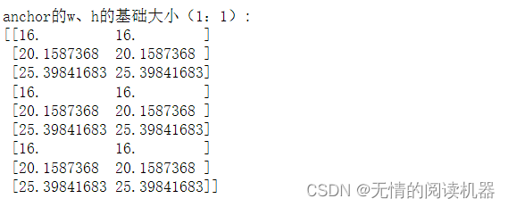
areas = anchors[:, 2] * anchors[:, 3]
print("基础面积:" )
print(areas)
anchors[:, 2] = np.sqrt(areas / np.repeat(ratios, len(scales)))
anchors[:, 3] = anchors[:, 2] * np.repeat(ratios, len(scales))
print("宽度:")
print(anchors[:, 2])
print("高度:")
print(anchors[:, 3])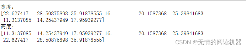
anchors[:, 0::2] -= np.tile(anchors[:, 2] * 0.5, (2, 1)).T
anchors[:, 1::2] -= np.tile(anchors[:, 3] * 0.5, (2, 1)).T
print("一个位置生成的anchor如下")
print("个数为:",anchors.shape[0] )
print(anchors)
2.为每个位置生成anchor
基本思想还是:anchor的生成都是以原图为基准的
想要实现上述思想,最重要的就是得到特征图与原图的缩放比例(步长),比如stride=8,那么如果原图大小为(image_w,image_h)那么特征图相对于原图尺寸就缩小为(image_w/8 , image_h/8)(计算结果是上采样的)
那么每个anchor的位置是由特征图决定的
x1∈( 0,1,2,3......image_w/8) y1∈( 0,1,2,3......image_h/8)
生成anchor的位置就是 c_x1 = x1+0.5 ,c_y1 = y1+0.5
因为anchor的生成是以原图为基准的,所以要将anchor在特征图的位置放大到原图,即在原图上生成anchor的位置是 c_x = c_x1 * stride , c_y = c_y1 * stride
def shift(shape, stride, anchors):shift_x = (np.arange(0, shape[1]) + 0.5) * strideshift_y = (np.arange(0, shape[0]) + 0.5) * strideshift_x, shift_y = np.meshgrid(shift_x, shift_y)shifts = np.vstack((shift_x.ravel(), shift_y.ravel(),shift_x.ravel(), shift_y.ravel())).transpose()# add A anchors (1, A, 4) to# cell K shifts (K, 1, 4) to get# shift anchors (K, A, 4)# reshape to (K*A, 4) shifted anchorsA = anchors.shape[0]K = shifts.shape[0]all_anchors = (anchors.reshape((1, A, 4)) + shifts.reshape((1, K, 4)).transpose((1, 0, 2)))all_anchors = all_anchors.reshape((K * A, 4))return all_anchors在代码层面上(anchors.reshape((1, A, 4)) + shifts.reshape((1, K, 4)).transpose((1, 0, 2)))
用到了向量相加的广播机制
向量a1维度是(k,1,4),含义是有K个位置,每个位置1份数据,每份数据4个参数(中心点)
向量a2维度是(1,A,4),含义是1个位置,每个位置A份数据,每份数据4个参数(anchor相对于中心点的位置坐标)
其中k是要在图像的k个位置上生成anchor,A是每个位置生成几个anchor
首先a2要在第0维复制k次(A,4)向量(为每个位置复制)
然后a1要在第1维复制A次(4)向下(为每个位置的每个anchor复制)
3.图片的anchor生成过程
最后输出的形状是 [1, 每层anchor数量之和 , 4]
class Anchors(nn.Module):def __init__(self, pyramid_levels=None, strides=None, sizes=None, ratios=None, scales=None):super(Anchors, self).__init__()#提取的特征if pyramid_levels is None:self.pyramid_levels = [3, 4, 5, 6, 7]#步长,在每层中,一个像素等于原始图像中几个像素if strides is None:self.strides = [2 ** x for x in self.pyramid_levels] #这个参数设置我没看懂#每层框子的基本边长if sizes is None:self.sizes = [2 ** (x + 2) for x in self.pyramid_levels] #这个参数设置我也没看懂#长宽比例if ratios is None:self.ratios = np.array([0.5, 1, 2])#边长缩放比例if scales is None:self.scales = np.array([2 ** 0, 2 ** (1.0 / 3.0), 2 ** (2.0 / 3.0)])def forward(self, image):#image是原图 shape为 batch,channel,w,h#这一步是获得宽和高image_shape = image.shape[2:]image_shape = np.array(image_shape)#‘//’是向下取整 整个式子相当于向上取整,因为不满1步的也要算1步#图像大小除以步长#在对应的每一层中,原图在该层对应的大小image_shapes = [(image_shape + 2 ** x - 1) // (2 ** x) for x in self.pyramid_levels]# 创建x1,y1 x2,y2 anchor的位置坐标all_anchors = np.zeros((0, 4)).astype(np.float32)for idx, p in enumerate(self.pyramid_levels):#传入该层anchor的基本边长,生成对应大小的anchoranchors = generate_anchors(base_size=self.sizes[idx], ratios=self.ratios, scales=self.scales)# 传入生成的anchor,和该层相对于原图的大小shifted_anchors = shift(image_shapes[idx], self.strides[idx], anchors)# 循环遍历完成之后,all_anchors的shape为 [每层anchor数量之和, 4]all_anchors = np.append(all_anchors, shifted_anchors, axis=0)# 最后输出的形状是 [1, 每层anchor数量之和 , 4]all_anchors = np.expand_dims(all_anchors, axis=0)if torch.cuda.is_available():return torch.from_numpy(all_anchors.astype(np.float32)).cuda()else:return torch.from_numpy(all_anchors.astype(np.float32))7.dataset
以csvdataset为例

相关文章:
Retinanet网络与focal loss损失
参考代码:https://github.com/yhenon/pytorch-retinanet 1.损失函数 1)原理 本文一个核心的贡献点就是 focal loss。总损失依然分为两部分,一部分是分类损失,一部分是回归损失。 在讲分类损失之前,我们来回顾一下二…...

Spring事务的失效场景
事务失效场景 方法用private或final修饰 Spring底层使用了AOP,而AOP的实现方式有两种,分别是JDK动态代理和CGLIB,JDK动态代理是实现抽象接口,CGLIB是继承父类,无论哪种方式,都需要重写方法来进行方法增强,而…...

芯动联科在科创板IPO过会:拟募资10亿元,金晓冬为实际控制人
2月13日,上海证券交易所披露的信息显示,安徽芯动联科微系统股份有限公司(下称“芯动联科”)获得科创板上市委会议审议通过。据贝多财经了解,芯动联科于2022年6月24日在科创板递交招股书。 本次冲刺上市,芯…...
数据结构之单链表
一、链表的组成 链表是由一个一个的节点组成的,节点又是一个一个的对象, 相邻的节点之间产生联系,形成一条链表。 例子:假如现在有两个人,A和B,A保存了B的联系方式,这俩人之间就有了联系。 A和…...

儿子跟妈妈关系不好怎么办?这里有解决办法!
15岁的男孩子正处于青春期,很多男孩都傲慢自大,听不进去别人的建议,以自己为中心,认为自己能处理好自己的事情,不想听父母的唠叨。母亲面对青春期的孩子也是举手无措,语气不好,会让孩子更叛逆。…...

论文投稿指南——中文核心期刊推荐(植物保护)
【前言】 🚀 想发论文怎么办?手把手教你论文如何投稿!那么,首先要搞懂投稿目标——论文期刊 🎄 在期刊论文的分布中,存在一种普遍现象:即对于某一特定的学科或专业来说,少数期刊所含…...

华科万维C++章节练习4_6
【程序设计】 题目: 编程输出下列图形,中间一行英文字母由输入得到。 A B B B C C C C C D D D D D D D C C C C C B B B A 开头空一格,字母间空两格…...

详解子网技术
一 : Internet地址 Intemet实质上是把分布在世界各地的各种网络如计算机局域网和广域网、数字数据通信网以及公用电话交换网等互相连接起来而形成的超级网络。但是 , 网络的物理地址给Internet统一全网地址带来两个方面的问题: 第一,物理地址是物理网络技术的一种…...
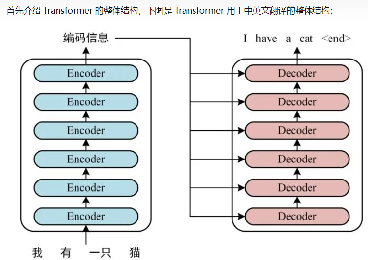
chatGTP的全称Chat Generative Pre-trained Transformer
chatGPT,有时候我会拼写为:chatGTP,所以知道这个GTP的全称是很有用的。 ChatGPT全名:Chat Generative Pre-trained Transformer ,中文翻译是:聊天生成预训练变压器,所以是GPT,G是生…...
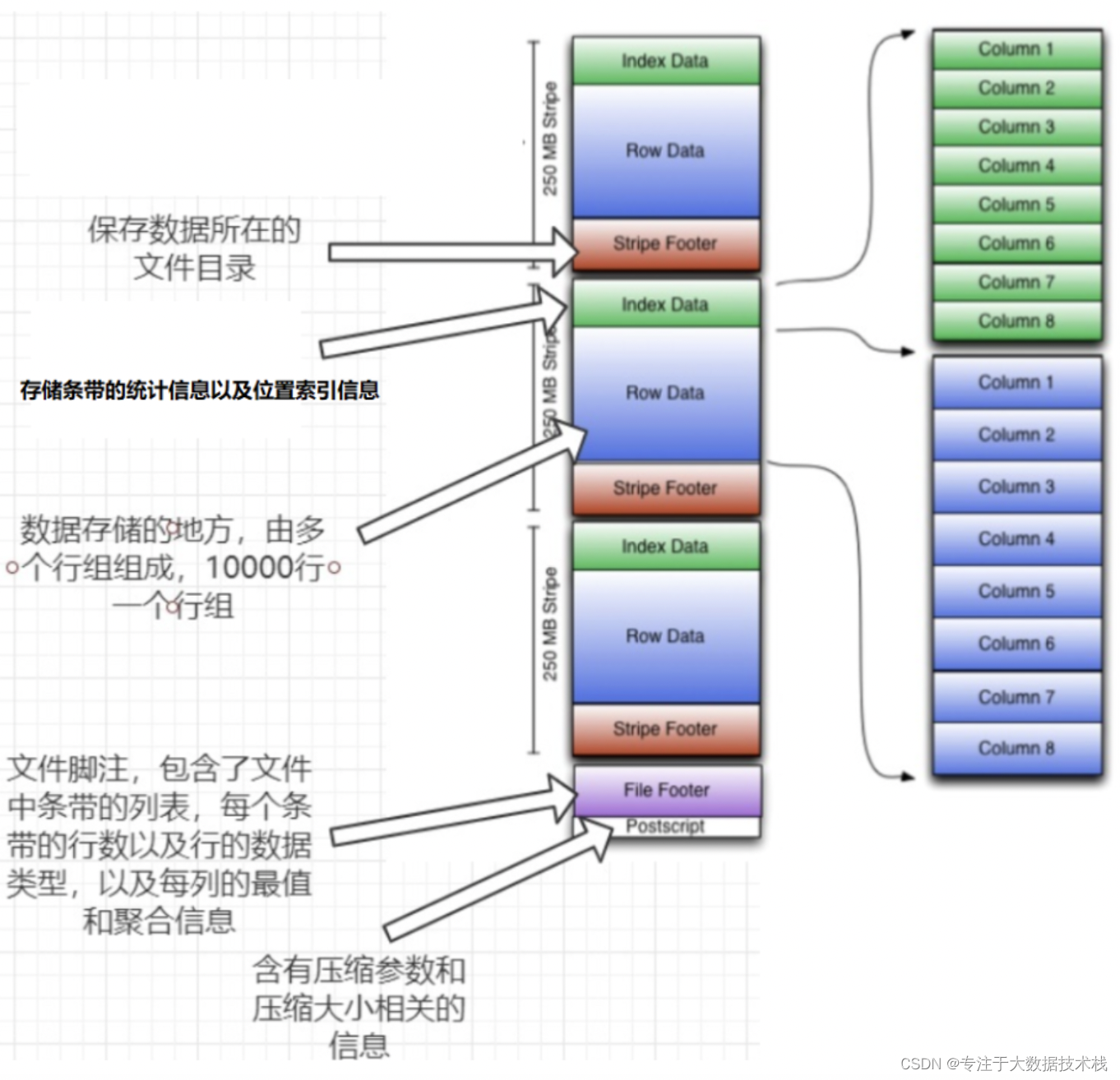
hive数据存储格式
1、Hive存储数据的格式如下: 存储数据格式存储形式TEXTFILE行式存储SEQUENCEFILE行式存储ORC列式存储PARQUET列式存储 2、行式存储和列式存储 解释: 1、上图左面为逻辑表;右面第一个为行式存储,第二个温列式存储; …...
mysql数据库备份与恢复
mysql数据备份: 数据备份方式 物理备份: 冷备:.冷备份指在数据库关闭后,进行备份,适用于所有模式的数据库热备:一般用于保证服务正常不间断运行,用两台机器作为服务机器,一台用于实际数据库操作应用,另外…...

《NFL橄榄球》:辛辛那提猛虎·橄榄1号位
辛辛那提猛虎(英语:Cincinnati Bengals),又译辛辛那提孟加拉虎,是一支职业美式橄榄球球队位于俄亥俄州辛辛那提。他们现时为美联北区的其中一支球队,他们在1968年加入美国橄榄球联合会,并在1970…...
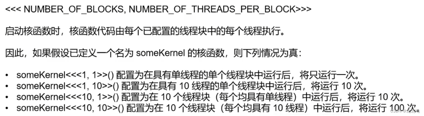
2、线程、块和网格
目录一、线程、块、网格概念二、代码分析2.1 打印第一个线程块的第一线程2.2 打印当前线程块的当前线程2.3 获取当前是第几个线程一、线程、块、网格概念 CUDA的软件架构由网格(Grid)、线程块(Block)和线程(Thread&am…...
C++ 算法主题系列之贪心算法的贪心之术
1. 前言 贪心算法是一种常见算法。是以人性之念的算法,面对众多选择时,总是趋利而行。 因贪心算法以眼前利益为先,故总能保证当前的选择是最好的,但无法时时保证最终的选择是最好的。当然,在局部利益最大化的同时&am…...
请注意,PDF正在传播恶意软件
据Bleeping Computer消息,安全研究人员发现了一种新型的恶意软件传播活动,攻击者通过使用PDF附件夹带恶意的Word文档,从而使用户感染恶意软件。 类似的恶意软件传播方式在以往可不多见。在大多数人的印象中,电子邮件是夹带加载了恶…...

【Kubernetes】【二】环境搭建 环境初始化
本章节主要介绍如何搭建kubernetes的集群环境 环境规划 集群类型 kubernetes集群大体上分为两类:一主多从和多主多从。 一主多从:一台Master节点和多台Node节点,搭建简单,但是有单机故障风险,适合用于测试环境多主…...
)
Python:每日一题之发现环(DFS)
题目描述 小明的实验室有 N 台电脑,编号 1⋯N。原本这 N 台电脑之间有 N−1 条数据链接相连,恰好构成一个树形网络。在树形网络上,任意两台电脑之间有唯一的路径相连。 不过在最近一次维护网络时,管理员误操作使得某两台电脑之间…...
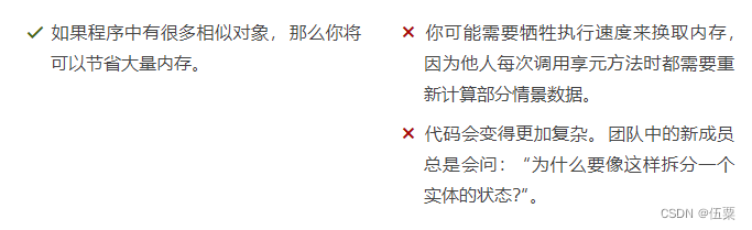
C++设计模式(14)——享元模式
亦称: 缓存、Cache、Flyweight 意图 享元模式是一种结构型设计模式, 它摒弃了在每个对象中保存所有数据的方式, 通过共享多个对象所共有的相同状态, 让你能在有限的内存容量中载入更多对象。 问题 假如你希望在长时间工作后放…...

SpringCloud之Eureka客户端服务启动报Cannot execute request on any known server解决
项目场景: 在练习SpringCloud时,Eureka客户端(client)出现报错:Cannot execute request on any known server 问题描述 正常启动SpringCloud的Server端和Client端,结果发现Server端的控制台有个Error提示,如下&#…...

从零开始搭建kubernetes集群环境(虚拟机/kubeadm方式)
文章目录1 Kubernetes简介(k8s)2 安装实战2.1 主机安装并初始化2.2 安装docker2.3 安装Kubernetes组件2.4 准备集群镜像2.5 集群初始化2.6 安装flannel网络插件3 部署nginx 测试3.1 创建一个nginx服务3.2 暴漏端口3.3 查看服务3.4 测试服务1 Kubernetes简…...
协议介绍)
IPv6之邻居发现(ND)协议介绍
引言 邻居发现协议(Neighbor Discovery Protocol,简称ND协议)是IPv6的一个关键协议,ND协议是IPv4一类协议在IPv6中综合起来的升级和改进,如ARP、ICMP路由器发现和ICMP重定向等协议。作为IPv6的基础性协议,ND还提供了其他功能,如前缀发现、邻居不可达检测、重复地址检测、…...

万物识别-中文镜像实际项目:校园安防图像中书包/水杯/运动器材识别
万物识别-中文镜像实际项目:校园安防图像中书包/水杯/运动器材识别 你有没有想过,学校里的监控摄像头除了看人,还能“看懂”画面里的东西?比如,识别出操场上遗落的书包、图书馆里被遗忘的水杯,或者体育馆里…...

实战指南:Kubernetes Dashboard的安装与高效管理
1. Kubernetes Dashboard入门指南 第一次接触Kubernetes Dashboard时,我被它简洁的UI界面惊艳到了。作为一个长期和命令行打交道的运维人员,终于不用再记那些复杂的kubectl命令了。Dashboard就像是给Kubernetes套上了一层可视化外衣,让集群管…...

从线性到非线性:PCA与KPCA的降维实战与核心差异
1. 降维技术的基本概念与需求 当你面对一份包含数百个特征的数据集时,第一反应可能是头疼。比如电商平台的用户行为数据,可能包含浏览记录、点击频率、停留时长、购买历史等数十个维度。这种高维数据不仅难以可视化,还会导致"维度灾难&q…...

基于OPC UA协议的PLC数据采集系统
在各级工业系统中,存在复杂的现场网络、多种总线和通信技术,各种设备的通信协议多种多样、解析标准各不相同,形成了数据孤岛;同时各类基于PC的控制和相关的可视化软件应用迅速增长,这些系统难以对接到复杂且孤立的协议…...

XMLView:浏览器端XML文档的智能解析与可视化解决方案
XMLView:浏览器端XML文档的智能解析与可视化解决方案 【免费下载链接】xmlview Powerful XML viewer for Google Chrome and Safari 项目地址: https://gitcode.com/gh_mirrors/xm/xmlview 面对复杂嵌套的XML文档时,您是否曾感到无从下手…...

PPI 以太网模块应用解析:S7-200 PLC 与上位机数据采集 + 触摸屏木材加工工艺报警系统配置
一、行业痛点在木材切割的锯片转速、进料速度、切割精度,以及木材拼接的压合压力、胶层厚度、拼接对齐度等工艺参数在线监测与控制领域,西门子 S7-200 系列 PLC 凭借抗干扰性强、编程便捷、适配工业现场的优势,成为中小型木材加工生产线控制核…...
)
从一次诡异的kubectl报错,聊聊K8s高可用架构中那些容易‘跑偏’的配置(HAProxy/Keepalived实战避坑)
从Kubectl报错透视Kubernetes高可用架构的七种致命配置误区 当kubectl get nodes返回"no route to host"时,大多数工程师的第一反应是检查kubeconfig文件——这没错,但可能错过背后更危险的架构隐患。去年我们生产环境就曾因HAProxy的TCP模式…...

MIPS寄存器文件设计避坑指南:从零开始用Logisim实现4x32位寄存器组
MIPS寄存器文件设计避坑指南:从零开始用Logisim实现4x32位寄存器组 在计算机体系结构的学习中,理解寄存器文件的工作原理是掌握CPU设计的关键一步。MIPS架构作为经典的RISC指令集,其寄存器文件设计体现了精简指令集的核心理念。本文将带您从零…...

COZE - 3
应用开发与发布 什么是应用? 通过扣子平台构建的 AI 应用具备强大的可扩展性,支持与个性化的用户界面绑定。扣子应用通过工作流或对话流处理复杂的业务逻辑与编排,其内置的丰富节点库提供了逻辑处理、知识写入与检索、大模型服务、会话管理等…...