机器学习笔记之优化算法(八)简单认识Wolfe Condition的收敛性证明
机器学习笔记之优化算法——简单认识Wolfe Condition收敛性证明
- 引言
引言
上一节介绍了非精确搜索方法—— Wolfe \text{Wolfe} Wolfe准则。本节将简单认识: Wolfe \text{Wolfe} Wolfe准则的收敛性证明。
回顾: Wolfe \text{Wolfe} Wolfe准则
关于先搜索方法表示如下:
x k + 1 = x k + α k ⋅ P k x_{k+1} = x_k + \alpha_k \cdot \mathcal P_k xk+1=xk+αk⋅Pk
在数值解迭代过程中,当前时刻的迭代步长结果 α k \alpha_k αk未确定的情况下,将步长设为变量 α \alpha α。在下降方向 P k \mathcal P_k Pk确定的条件下,关于 x k + 1 x_{k+1} xk+1的目标函数结果 f ( x k + 1 ) f(x_{k+1}) f(xk+1)可表示为关于变量 α \alpha α的函数 ϕ ( α ) \phi(\alpha) ϕ(α):
f ( x k + 1 ) = f ( x k + α ⋅ P k ) = ϕ ( α ) f(x_{k+1}) = f(x_k + \alpha \cdot \mathcal P_k) = \phi(\alpha) f(xk+1)=f(xk+α⋅Pk)=ϕ(α)
由于 { f ( x k ) } k = 0 ∞ \{f(x_k)\}_{k=0}^{\infty} {f(xk)}k=0∞服从严格的单调性仅是目标函数收敛至最优解: { f ( x k ) } k = 0 ∞ ⇒ f ∗ \{f(x_k)\}_{k=0}^{\infty} \Rightarrow f^* {f(xk)}k=0∞⇒f∗的必要不充分条件;因而需要相比更严格的条件使目标函数收敛至最优解: Armijo \text{Armijo} Armijo准则、 Glodstein \text{Glodstein} Glodstein准则与 Wolfe \text{Wolfe} Wolfe准则:
Armijo Condition : { ϕ ( α ) < f ( x k ) + C 1 ⋅ [ ∇ f ( x k ) ] T P k ⋅ α C 1 ∈ ( 0 , 1 ) Glodstein Condition : { f ( x k ) + ( 1 − C ) ⋅ [ ∇ f ( x k ) ] T P k ⋅ α ≤ ϕ ( α ) ≤ f ( x k ) + C ⋅ [ ∇ f ( x k ) ] T P k ⋅ α C ∈ ( 0 , 1 2 ) \begin{aligned} & \text{Armijo Condition : } \begin{cases} \phi(\alpha) < f(x_k) + \mathcal C_1 \cdot [\nabla f(x_k)]^T \mathcal P_k \cdot \alpha \\ \quad \\ \mathcal C_1 \in (0,1) \end{cases} \\ & \text{Glodstein Condition : } \begin{cases} f(x_k) + (1 - \mathcal C) \cdot [\nabla f(x_k)]^T \mathcal P_k \cdot \alpha \leq \phi(\alpha) \leq f(x_k) + \mathcal C \cdot [\nabla f(x_k)]^T \mathcal P_k \cdot \alpha \\ \quad \\ \mathcal C \in \begin{aligned}\left(0,\frac{1}{2}\right)\end{aligned} \end{cases} \end{aligned} Armijo Condition : ⎩ ⎨ ⎧ϕ(α)<f(xk)+C1⋅[∇f(xk)]TPk⋅αC1∈(0,1)Glodstein Condition : ⎩ ⎨ ⎧f(xk)+(1−C)⋅[∇f(xk)]TPk⋅α≤ϕ(α)≤f(xk)+C⋅[∇f(xk)]TPk⋅αC∈(0,21)
而 Wolfe \text{Wolfe} Wolfe准则的初衷是为了处理 Armijo \text{Armijo} Armijo准则与 Goldstein \text{Goldstein} Goldstein准则的共同弊端:仅通过划分边界 ( Armijo ) (\text{Armijo}) (Armijo)或者划分边界构成的范围 ( Glodstein ) (\text{Glodstein}) (Glodstein)对相应的 α \alpha α结果进行筛选,而被选择的 α \alpha α结果是否存在意义 ? ? ? 未知。
基于上述因素, Wlofe \text{Wlofe} Wlofe准则在 Armijo \text{Armijo} Armijo准则的基础上,建立软性规则以筛选优质的 α \alpha α结果:
其中 ϕ ′ ( α ) = ∂ f ( x k + α ⋅ P k ) ∂ α = [ ∇ f ( x k + α ⋅ P k ) ] T P k \begin{aligned}\phi'(\alpha) = \frac{\partial f(x_k + \alpha \cdot \mathcal P_k)}{\partial \alpha} = \left[\nabla f(x_k + \alpha \cdot \mathcal P_k)\right]^T \mathcal P_k \end{aligned} ϕ′(α)=∂α∂f(xk+α⋅Pk)=[∇f(xk+α⋅Pk)]TPk。
{ ϕ ( α ) ≤ f ( x k ) + C 1 ⋅ [ ∇ f ( x k ) ] T P k ⋅ α ϕ ′ ( α ) ≥ C 2 ⋅ [ ∇ f ( x k ) ] T P k C 1 ∈ ( 0 , 1 ) C 2 ∈ ( C 1 , 1 ) \begin{cases} \phi(\alpha) \leq f(x_k) +\mathcal C_1 \cdot [\nabla f(x_k)]^T \mathcal P_k \cdot \alpha \\ \phi'(\alpha) \geq \mathcal C_2 \cdot [\nabla f(x_k)]^T \mathcal P_k \\ \mathcal C_1 \in (0,1) \\ \mathcal C_2 \in (\mathcal C_1,1) \end{cases} ⎩ ⎨ ⎧ϕ(α)≤f(xk)+C1⋅[∇f(xk)]TPk⋅αϕ′(α)≥C2⋅[∇f(xk)]TPkC1∈(0,1)C2∈(C1,1)
本节以 Wolfe \text{Wolfe} Wolfe准则为例,简单介绍该准则的收敛性证明。
准备工作
推导条件介绍
-
关于目标函数优化的终极目标: min X ∈ R n f ( X ) \mathop{\min}\limits_{\mathcal X \in \mathbb R^n} f(\mathcal X) X∈Rnminf(X),因而对于目标函数 f ( X ) f(\mathcal X) f(X),需要满足:向下有界,并且在定义域内连续可微;
这属于函数自身的性质,在迭代过程中不能无限地小下去。 -
关于 f ( X ) f(\mathcal X) f(X)的梯度函数 ∇ f ( X ) \nabla f(\mathcal X) ∇f(X),需要在定义域内满足利普希茨连续 ( Lipschitz Continuity ) (\text{Lipschitz Continuity}) (Lipschitz Continuity)。对应数学符号表示如下:
其中L \mathcal L L是一个常数。
∀ x , x ^ ∈ R n , ∃ L : s . t . ∣ ∣ ∇ f ( x ) − ∇ f ( x ^ ) ∣ ∣ ≤ L ⋅ ∣ ∣ x − x ^ ∣ ∣ \forall x,\hat x \in \mathbb R^n, \exist \mathcal L :\quad s.t. ||\nabla f(x) - \nabla f(\hat x)|| \leq \mathcal L \cdot ||x - \hat x|| ∀x,x^∈Rn,∃L:s.t.∣∣∇f(x)−∇f(x^)∣∣≤L⋅∣∣x−x^∣∣
如果一个普通函数 G ( x ) \mathcal G(x) G(x)满足利普希兹连续,可以将上述描述使用 G ( x ) \mathcal G(x) G(x)进行替换,并进行简单变换:
∣ ∣ G ( x ) − G ( x ^ ) ∣ ∣ ≤ L ⋅ ∣ ∣ x − x ^ ∣ ∣ ⇒ ∣ ∣ G ( x ) − G ( x ^ ) x − x ^ ∣ ∣ ≤ L ||\mathcal G(x) - \mathcal G(\hat x)|| \leq \mathcal L \cdot ||x - \hat x|| \Rightarrow \left|\left|\frac{\mathcal G(x) - \mathcal G(\hat x)}{x - \hat x}\right|\right| \leq \mathcal L ∣∣G(x)−G(x^)∣∣≤L⋅∣∣x−x^∣∣⇒ x−x^G(x)−G(x^) ≤L
关于小于号左侧的式子格式: ∣ ∣ G ( x ) − G ( x ^ ) x − x ^ ∣ ∣ \begin{aligned}\left|\left|\frac{\mathcal G(x) - \mathcal G(\hat x)}{x - \hat x}\right|\right|\end{aligned} x−x^G(x)−G(x^) ,根据拉格朗日中值定理,可将该式表示为如下形式:
∃ ξ ∈ ( x , x ^ ) ⇒ ∣ ∣ G ( x ) − G ( x ^ ) x − x ^ ∣ ∣ = G ′ ( ξ ) \exist \xi \in (x,\hat x) \Rightarrow \begin{aligned}\left|\left|\frac{\mathcal G(x) - \mathcal G(\hat x)}{x - \hat x}\right|\right|\end{aligned} = \mathcal G'(\xi) ∃ξ∈(x,x^)⇒ x−x^G(x)−G(x^) =G′(ξ)
从而将利普希兹连续描述为如下形式:
∃ ξ ∈ ( x , x ^ ) ⇒ ∣ ∣ G ′ ( ξ ) ∣ ∣ ≤ L \exist \xi \in (x,\hat x) \Rightarrow ||\mathcal G'(\xi)|| \leq \mathcal L ∃ξ∈(x,x^)⇒∣∣G′(ξ)∣∣≤L
这意味着(不严谨):关于函数 G ( x ) \mathcal G(x) G(x)的一阶导函数 G ′ ( x ) \mathcal G'(x) G′(x)存在上界 L \mathcal L L。回到条件中,关于 ∇ f ( X ) \nabla f(\mathcal X) ∇f(X)服从利普希兹连续可理解为:对目标函数的二阶梯度结果进行约束:
∂ ∇ f ( X ) ∂ X ≤ L \begin{aligned}\frac{\partial \nabla f(\mathcal X)}{\partial \mathcal X}\end{aligned} \leq \mathcal L ∂X∂∇f(X)≤L
根据二阶梯度的几何意义,该条件本质上是对目标函数 f ( X ) f(\mathcal X) f(X)中斜率的变化量进行约束。关于不满足利普希兹连续的函数示例: f ( x ) = x 2 f(x) = x^2 f(x)=x2。对应函数图像表示如下:

关于该函数的一阶导函数 ∂ f ∂ x = 2 x \begin{aligned}\frac{\partial f}{\partial x} = 2x\end{aligned} ∂x∂f=2x,是一个关于 x x x的一次函数,在定义域 x ∈ R x \in \mathbb R x∈R中,其并不受某常数 L \mathcal L L的约束。
当x ⇒ ∞ x \Rightarrow \infty x⇒∞时,对应的∂ f ∂ x ⇒ ∞ \begin{aligned}\frac{\partial f}{\partial x} \Rightarrow \infty \end{aligned} ∂x∂f⇒∞。
再如: f ( x ) = 1 x \begin{aligned}f(x) = \frac{1}{x}\end{aligned} f(x)=x1。对应函数图像表示如下:

同理,关于该函数的一阶导函数 ∂ f ∂ x = − 1 x 2 \begin{aligned}\frac{\partial f}{\partial x} = -\frac{1}{x^2}\end{aligned} ∂x∂f=−x21,在其定义域 x > 0 x > 0 x>0中,其同样不受某常数 L \mathcal L L的约束。
当x ⇒ 0 x \Rightarrow 0 x⇒0时,对应的∂ f ∂ x = − ∞ \begin{aligned}\frac{\partial f}{\partial x} = -\infty\end{aligned} ∂x∂f=−∞。
可以看出:上述两个例子在其对应的定义域内均是连续的,但它们不满足利普希兹连续。也就是说:利普希兹连续的条件更强。
关于连续相关概念按照条件强度对比表示为:连续 < < < 一致连续 < < < 利普希兹连续(利普希兹条件)。上述条件强度可理解为:
若某函数在其定义域内满足利普希兹连续,那么该函数一定满足一致连续和连续,反之不行;
同理,若某函数在其定义域内满足一致连续,那么该函数一定满足连续,反之不行。其中一致连续与连续之间的区别可描述为:连续仅要求函数在其定义域内没有断点或者跳跃的情况;而一致连续在没有断点或者跳跃的基础上,还需要满足:函数 f ( ⋅ ) f(\cdot) f(⋅)在定义域内任意的两个点 x 、 y x、y x、y,如果 x x x与 y y y充分接近时,对应的 f ( x ) f(x) f(x)与 f ( y ) f(y) f(y)也要充分接近。很明显,上例中的f ( x ) = 1 x \begin{aligned}f(x) = \frac{1}{x}\end{aligned} f(x)=x1就不是一致连续:首先 f ( x ) f(x) f(x)在其定义域 ( 0 , + ∞ ) (0,+\infty) (0,+∞)中连续,但如果选择无限靠近 0 0 0的两个比较接近的点,它们的函数值并不充分接近 ( ∞ ) (\infty) (∞)。
-
条件 3 3 3: P k \mathcal P_k Pk是下降方向 ( Descent Direction ) (\text{Descent Direction}) (Descent Direction)。
这里使用的是更加泛化的‘下降方向’,而不仅仅是最速下降方向。其在非精确搜索方法中被确定下的。关于下降方向详见线搜索方法——精确搜索。
P k \mathcal P_k Pk作为下降方向,必然有:
− [ ∇ f ( x k ) ] T P k = ∣ ∣ ∇ f ( x k ) ∣ ∣ ⋅ ∣ P k ∣ ∣ cos θ k > 0 - [\nabla f(x_k)]^T \mathcal P_k = ||\nabla f(x_k)|| \cdot |\mathcal P_k|| \cos \theta_k> 0 −[∇f(xk)]TPk=∣∣∇f(xk)∣∣⋅∣Pk∣∣cosθk>0
其中 θ k \theta_k θk是负梯度方向 − ∇ f ( x k ) -\nabla f(x_k) −∇f(xk)与下降方向 P k \mathcal P_k Pk之间的夹角,因而该夹角的范围必然在 ( − π 2 , π 2 ) \begin{aligned}\left(-\frac{\pi}{2},\frac{\pi}{2}\right)\end{aligned} (−2π,2π)之间。也就是说: cos θ k > 0 \cos \theta_k >0 cosθk>0恒成立:
也可以理解为− ∇ f ( x k ) -\nabla f(x_k) −∇f(xk)与P k \mathcal P_k Pk两者之间的夹角是锐角(没有先后顺序),对应的范围是( 0 , π 2 ) \begin{aligned}\left(0,\frac{\pi}{2}\right)\end{aligned} (0,2π)。
cos θ k = − [ ∇ f ( x k ) ] T P k ∣ ∣ ∇ f ( x k ) ∣ ∣ ⋅ ∣ ∣ P k ∣ ∣ > 0 \begin{aligned} \cos \theta_k = \frac{-[\nabla f(x_k)]^T \mathcal P_k}{||\nabla f(x_k)||\cdot ||\mathcal P_k||} > 0 \end{aligned} cosθk=∣∣∇f(xk)∣∣⋅∣∣Pk∣∣−[∇f(xk)]TPk>0 -
迭代过程中的最优步长 α k ( k = 1 , 2 , 3 , ⋯ ) \alpha_k(k=1,2,3,\cdots) αk(k=1,2,3,⋯)满足 Wolfe \text{Wolfe} Wolfe准则:
该条件不再赘述。
{ f ( x k + 1 ) < f ( x k ) + C 1 ⋅ [ ∇ f ( x k ) ] T P k ⋅ α k [ ∇ f ( x k + 1 ) ] T P k ≥ C 2 ⋅ [ ∇ f ( x k ) ] T P k C 1 ∈ ( 0 , 1 ) C 2 ∈ ( C 1 , 1 ) \begin{cases} f(x_{k+1}) < f(x_k) + \mathcal C_1 \cdot [\nabla f(x_k)]^T \mathcal P_k \cdot \alpha_k \\ [\nabla f(x_{k+1})]^T \mathcal P_k \geq \mathcal C_2 \cdot [\nabla f(x_k)]^T \mathcal P_k \\ \mathcal C_1 \in (0,1) \\ \mathcal C_2 \in (\mathcal C_1,1) \end{cases} ⎩ ⎨ ⎧f(xk+1)<f(xk)+C1⋅[∇f(xk)]TPk⋅αk[∇f(xk+1)]TPk≥C2⋅[∇f(xk)]TPkC1∈(0,1)C2∈(C1,1)
推导结论介绍
关于最终需要证明的收敛性,自然是数值解序列 { x k } k = 0 ∞ \{x_k\}_{k=0}^{\infty} {xk}k=0∞对应的目标函数结果 { f ( x k ) } k = 0 ∞ \{f(x_k)\}_{k=0}^{\infty} {f(xk)}k=0∞收敛到某最优解 f ∗ f^* f∗:
{ f ( x k ) } k = 0 ∞ ⇒ f ∗ \{f(x_k)\}_{k=0}^{\infty} \Rightarrow f^* {f(xk)}k=0∞⇒f∗
如果从梯度的角度观察,关于数值解序列对应的目标函数梯度结果 { ∇ f ( x k ) } k = 0 ∞ \{\nabla f(x_k)\}_{k=0}^{\infty} {∇f(xk)}k=0∞收敛到 0 0 0即可:
常数函数对应的梯度范数就是 0 0 0。
lim k ⇒ + ∞ ∣ ∣ ∇ f ( x k ) ∣ ∣ = 0 \mathop{\lim}\limits_{k \Rightarrow + \infty} ||\nabla f(x_k)|| = 0 k⇒+∞lim∣∣∇f(xk)∣∣=0
根据上面关于 θ k \theta_k θk的描述,将其控制为:
[ cos θ k ] 2 ≥ η [\cos \theta_k]^2 \geq \eta [cosθk]2≥η
其中 η \eta η表示一个 > 0 > 0 >0的小的常数。基于此,关于 ∑ k = 0 ∞ [ cos θ k ] 2 \begin{aligned}\sum_{k=0}^{\infty} [\cos \theta_k]^2\end{aligned} k=0∑∞[cosθk]2的结果必定是发散的。也就是说: + ∞ +\infty +∞个 > 0 >0 >0的较小常数相加必然还是 + ∞ +\infty +∞。
∑ k = 0 + ∞ [ cos θ k ] 2 = + ∞ \sum_{k=0}^{+\infty} [\cos \theta_k]^2 = +\infty k=0∑+∞[cosθk]2=+∞
如果将推导结论设置为如下形式:
∑ k = 0 + ∞ [ cos θ k ] 2 ⋅ ∣ ∣ ∇ f ( x k ) ∣ ∣ 2 < + ∞ \sum_{k=0}^{+\infty} [\cos \theta_k]^2 \cdot ||\nabla f(x_k)||^2 < +\infty k=0∑+∞[cosθk]2⋅∣∣∇f(xk)∣∣2<+∞
那么该式子必然等价于:
之所以等价是因为上式中的项 ∑ k = 0 + ∞ [ cos θ k ] 2 ⋅ ∣ ∣ ∇ f ( x k ) ∣ ∣ 2 \sum_{k=0}^{+\infty} [\cos \theta_k]^2 \cdot ||\nabla f(x_k)||^2 ∑k=0+∞[cosθk]2⋅∣∣∇f(xk)∣∣2与关于 cos θ k \cos \theta_k cosθk的项 ∑ k = 0 + ∞ [ cos θ k ] 2 \sum_{k=0}^{+\infty} [\cos \theta_k]^2 ∑k=0+∞[cosθk]2相矛盾。这只有一种解释:
随着k k k值的增加,使得lim k ⇒ + ∞ ∣ ∣ ∇ f ( x k ) ∣ ∣ = 0 \mathop{\lim}\limits_{k \Rightarrow +\infty} ||\nabla f(x_k)|| = 0 k⇒+∞lim∣∣∇f(xk)∣∣=0;从而使lim k ⇒ + ∞ ∣ ∣ ∇ f ( x k ) ∣ ∣ 2 = 0 \mathop{\lim}\limits_{k \Rightarrow +\infty} ||\nabla f(x_k)||^2 = 0 k⇒+∞lim∣∣∇f(xk)∣∣2=0;从而使lim k ⇒ + ∞ [ cos θ k ] 2 ⋅ ∣ ∣ ∇ f ( x k ) ∣ ∣ 2 < lim k ⇒ + ∞ [ cos θ k ] 2 = η \mathop{\lim}\limits_{k \Rightarrow +\infty}[\cos \theta_k]^2 \cdot ||\nabla f(x_k)||^2 < \mathop{\lim}\limits_{k \Rightarrow +\infty} [\cos \theta_k]^2 = \eta k⇒+∞lim[cosθk]2⋅∣∣∇f(xk)∣∣2<k⇒+∞lim[cosθk]2=η最终使∑ k = 0 + ∞ [ cos θ k ] 2 ⋅ ∣ ∣ ∇ f ( x k ) ∣ ∣ 2 < ∑ k = 0 + ∞ [ cos θ k ] 2 = + ∞ \sum_{k=0}^{+\infty} [\cos \theta_k]^2 \cdot ||\nabla f(x_k)||^2 < \sum_{k=0}^{+\infty}[\cos \theta_k]^2 = +\infty ∑k=0+∞[cosθk]2⋅∣∣∇f(xk)∣∣2<∑k=0+∞[cosθk]2=+∞
∑ k = 0 + ∞ [ cos θ k ] 2 ⋅ ∣ ∣ ∇ f ( x k ) ∣ ∣ 2 < + ∞ ⇔ lim k ⇒ ∞ ∣ ∣ ∇ f ( x k ) ∣ ∣ = 0 \sum_{k=0}^{+\infty} [\cos \theta_k]^2 \cdot ||\nabla f(x_k)||^2 < +\infty \Leftrightarrow \lim_{k \Rightarrow \infty} ||\nabla f(x_k)|| = 0 k=0∑+∞[cosθk]2⋅∣∣∇f(xk)∣∣2<+∞⇔k⇒∞lim∣∣∇f(xk)∣∣=0
最终可以描述出 { f ( x k ) } k = 0 ∞ \{f(x_k)\}_{k=0}^{\infty} {f(xk)}k=0∞可以收敛到最优解。
关于 Wolfe \text{Wolfe} Wolfe准则收敛性证明的推导过程
证明:
-
基于 Wolfe \text{Wolfe} Wolfe准则中的 [ ∇ f ( x k + 1 ) ] T P k ≥ C 2 ⋅ [ ∇ f ( x k ) ] T P k [\nabla f(x_{k+1})]^T \mathcal P_k \geq \mathcal C_2 \cdot [\nabla f(x_k)]^T \mathcal P_k [∇f(xk+1)]TPk≥C2⋅[∇f(xk)]TPk,将不等式两端同时减去 [ ∇ f ( x k ) ] T P k [\nabla f(x_k)]^T \mathcal P_k [∇f(xk)]TPk,目的是凑出利普希兹条件:
[ ∇ f ( x k + 1 ) ] T P k − [ ∇ f ( x k ) ] T P k ≥ C 2 ⋅ [ ∇ f ( x k ) ] T P k − [ ∇ f ( x k ) ] T P k ⇒ { [ ∇ f ( x k + 1 ) ] − [ ∇ f ( x k ) ] } T P k ≥ ( C 2 − 1 ) ⋅ [ ∇ f ( x k ) ] T P k \begin{aligned} & \quad [\nabla f(x_{k+1})]^T \mathcal P_k - [\nabla f(x_k)]^T \mathcal P_k \geq \mathcal C_2 \cdot [\nabla f(x_k)]^T \mathcal P_k - [\nabla f(x_k)]^T \mathcal P_k \\ & \Rightarrow \left\{ [\nabla f(x_{k+1})] - [\nabla f(x_k)] \right\}^T \mathcal P_k \geq (\mathcal C_2 -1) \cdot [\nabla f(x_k)]^T \mathcal P_k \end{aligned} [∇f(xk+1)]TPk−[∇f(xk)]TPk≥C2⋅[∇f(xk)]TPk−[∇f(xk)]TPk⇒{[∇f(xk+1)]−[∇f(xk)]}TPk≥(C2−1)⋅[∇f(xk)]TPk
观察不等式左侧,可以将 { [ ∇ f ( x k + 1 ) ] − [ ∇ f ( x k ) ] } T P k \left\{ [\nabla f(x_{k+1})] - [\nabla f(x_k)] \right\}^T \mathcal P_k {[∇f(xk+1)]−[∇f(xk)]}TPk视作两个向量之间的内积。基于此,必然满足如下表达:
因为cos θ \cos \theta cosθ的值域是[ − 1 , 1 ] [-1,1] [−1,1]。其中θ \theta θ表示向量[ ∇ f ( x k + 1 ) ] − [ ∇ f ( x k ) ] [\nabla f(x_{k+1})] - [\nabla f(x_k)] [∇f(xk+1)]−[∇f(xk)]与向量P k \mathcal P_k Pk之间的夹角。
{ [ ∇ f ( x k + 1 ) ] − [ ∇ f ( x k ) ] } T P k = ∣ ∣ [ ∇ f ( x k + 1 ) ] − [ ∇ f ( x k ) ] ∣ ∣ ⋅ ∣ ∣ P k ∣ ∣ ⋅ cos θ ∣ ∣ [ ∇ f ( x k + 1 ) ] − [ ∇ f ( x k ) ] ∣ ∣ ⋅ ∣ ∣ P k ∣ ∣ ⋅ cos θ ≤ ∣ ∣ [ ∇ f ( x k + 1 ) ] − [ ∇ f ( x k ) ] ∣ ∣ ⋅ ∣ ∣ P k ∣ ∣ \left\{ [\nabla f(x_{k+1})] - [\nabla f(x_k)] \right\}^T \mathcal P_k = ||[\nabla f(x_{k+1})] - [\nabla f(x_k)]|| \cdot ||\mathcal P_k|| \cdot \cos \theta \\ \quad \\ ||[\nabla f(x_{k+1})] - [\nabla f(x_k)]|| \cdot ||\mathcal P_k|| \cdot \cos \theta \leq ||[\nabla f(x_{k+1})] - [\nabla f(x_k)]|| \cdot ||\mathcal P_k|| {[∇f(xk+1)]−[∇f(xk)]}TPk=∣∣[∇f(xk+1)]−[∇f(xk)]∣∣⋅∣∣Pk∣∣⋅cosθ∣∣[∇f(xk+1)]−[∇f(xk)]∣∣⋅∣∣Pk∣∣⋅cosθ≤∣∣[∇f(xk+1)]−[∇f(xk)]∣∣⋅∣∣Pk∣∣
综上,可将式子整理为:
∣ ∣ [ ∇ f ( x k + 1 ) ] − [ ∇ f ( x k ) ] ∣ ∣ ⋅ ∣ ∣ P k ∣ ∣ ≥ { [ ∇ f ( x k + 1 ) ] − [ ∇ f ( x k ) ] } T P k ≥ ( C 2 − 1 ) ⋅ [ ∇ f ( x k ) ] T P k ||[\nabla f(x_{k+1})] - [\nabla f(x_k)]|| \cdot ||\mathcal P_k|| \geq \left\{ [\nabla f(x_{k+1})] - [\nabla f(x_k)] \right\}^T \mathcal P_k \geq (\mathcal C_2 -1) \cdot [\nabla f(x_k)]^T \mathcal P_k ∣∣[∇f(xk+1)]−[∇f(xk)]∣∣⋅∣∣Pk∣∣≥{[∇f(xk+1)]−[∇f(xk)]}TPk≥(C2−1)⋅[∇f(xk)]TPk -
观察式子 ∣ ∣ [ ∇ f ( x k + 1 ) ] − [ ∇ f ( x k ) ] ∣ ∣ ⋅ ∣ ∣ P k ∣ ∣ ||[\nabla f(x_{k+1})] - [\nabla f(x_k)]|| \cdot ||\mathcal P_k|| ∣∣[∇f(xk+1)]−[∇f(xk)]∣∣⋅∣∣Pk∣∣,使用利普希兹条件将其转化为:
其中L \mathcal L L是利普希兹条件中的常数;将x k + 1 = x k + α k ⋅ P k x_{k+1} = x_k + \alpha_k \cdot \mathcal P_k xk+1=xk+αk⋅Pk代入。
∣ ∣ [ ∇ f ( x k + 1 ) ] − [ ∇ f ( x k ) ] ∣ ∣ ⋅ ∣ ∣ P k ∣ ∣ ≤ L ⋅ ∣ ∣ x k + 1 − x k ∣ ∣ ⋅ ∣ ∣ P k ∣ ∣ = L ⋅ ∣ ∣ α k ⋅ P k ∣ ∣ ⋅ ∣ ∣ P k ∣ ∣ = L ⋅ α k ⋅ ∣ ∣ P k ∣ ∣ 2 \begin{aligned} ||[\nabla f(x_{k+1})] - [\nabla f(x_k)]|| \cdot ||\mathcal P_k|| & \leq \mathcal L \cdot ||x_{k+1} - x_k|| \cdot ||\mathcal P_k||\\ & = \mathcal L \cdot ||\alpha_k \cdot \mathcal P_k|| \cdot ||\mathcal P_k||\\ & = \mathcal L \cdot \alpha_k \cdot ||\mathcal P_k||^2 \end{aligned} ∣∣[∇f(xk+1)]−[∇f(xk)]∣∣⋅∣∣Pk∣∣≤L⋅∣∣xk+1−xk∣∣⋅∣∣Pk∣∣=L⋅∣∣αk⋅Pk∣∣⋅∣∣Pk∣∣=L⋅αk⋅∣∣Pk∣∣2
至此,可以得到式子:
由于α k , ∣ ∣ P k ∣ ∣ 2 \alpha_k,||\mathcal P_k||^2 αk,∣∣Pk∣∣2均恒正;且不等式右侧C 2 − 1 < 0 , [ ∇ f ( x k ) ] T P k < 0 \mathcal C_2 -1 <0,[\nabla f(x_k)]^T \mathcal P_k <0 C2−1<0,[∇f(xk)]TPk<0恒成立;因此L \mathcal L L必然是一个> 0 >0 >0的值。
L ⋅ α k ⋅ ∣ ∣ P k ∣ ∣ 2 ≥ ( C 2 − 1 ) ⋅ [ ∇ f ( x k ) ] T P k \mathcal L \cdot \alpha_k \cdot ||\mathcal P_k||^2 \geq (\mathcal C_2 -1) \cdot [\nabla f(x_k)]^T \mathcal P_k L⋅αk⋅∣∣Pk∣∣2≥(C2−1)⋅[∇f(xk)]TPk
将 L , ∣ ∣ P k ∣ ∣ 2 \mathcal L,||\mathcal P_k||^2 L,∣∣Pk∣∣2移到大于等于号右侧,符号不发生变化:
α k ≥ C 2 − 1 L ⋅ [ ∇ f ( x k ) ] T P k ∣ ∣ P k ∣ ∣ 2 \alpha_k \geq \frac{\mathcal C_2 - 1}{\mathcal L} \cdot \frac{[\nabla f(x_k)]^T \mathcal P_k}{||\mathcal P_k||^2} αk≥LC2−1⋅∣∣Pk∣∣2[∇f(xk)]TPk -
至此,将上式与 Wolfe \text{Wolfe} Wolfe准则的第一项关联起来:
由于C 1 ⋅ [ ∇ f ( x k ) ] T P k < 0 \mathcal C_1 \cdot [\nabla f(x_k)]^T \mathcal P_k < 0 C1⋅[∇f(xk)]TPk<0那么将上式代入,必然有:
就是‘负的不那么厉害了~’
C 1 ⋅ [ ∇ f ( x k ) ] T P k ⋅ ( C 2 − 1 L ⋅ [ ∇ f ( x k ) ] T P k ∣ ∣ P k ∣ ∣ 2 ) ≥ C 1 ⋅ [ ∇ f ( x k ) ] T P k ⋅ α k \mathcal C_1 \cdot [\nabla f(x_k)]^T \mathcal P_k \cdot \left(\frac{\mathcal C_2 - 1}{\mathcal L} \cdot \frac{[\nabla f(x_k)]^T \mathcal P_k}{||\mathcal P_k||^2}\right) \geq \mathcal C_1 \cdot [\nabla f(x_k)]^T \mathcal P_k \cdot \alpha_k C1⋅[∇f(xk)]TPk⋅(LC2−1⋅∣∣Pk∣∣2[∇f(xk)]TPk)≥C1⋅[∇f(xk)]TPk⋅αk
从而有:
f ( x k + 1 ) ≤ f ( x k ) + C 1 ⋅ [ ∇ f ( x k ) ] T P k ⋅ ( C 2 − 1 L ⋅ [ ∇ f ( x k ) ] T P k ∣ ∣ P k ∣ ∣ 2 ) f(x_{k+1}) \leq f(x_k) + \mathcal C_1 \cdot [\nabla f(x_k)]^T \mathcal P_k \cdot \left(\frac{\mathcal C_2 - 1}{\mathcal L} \cdot \frac{[\nabla f(x_k)]^T \mathcal P_k}{||\mathcal P_k||^2}\right) f(xk+1)≤f(xk)+C1⋅[∇f(xk)]TPk⋅(LC2−1⋅∣∣Pk∣∣2[∇f(xk)]TPk)
观察小于等于号右侧后一项:将其描述成分式形式,会包含一个关于 [ ∇ f ( x k ) ] T P k [\nabla f(x_k)]^T \mathcal P_k [∇f(xk)]TPk的平方项,因此使用 [ ∇ f ( x k ) ] T P k = − ∣ ∣ ∇ f ( x k ) ∣ ∣ ⋅ ∣ ∣ P k ∣ ∣ ⋅ cos θ k [\nabla f(x_k)]^T \mathcal P_k = -||\nabla f(x_k)|| \cdot ||\mathcal P_k|| \cdot \cos \theta_k [∇f(xk)]TPk=−∣∣∇f(xk)∣∣⋅∣∣Pk∣∣⋅cosθk进行替换:其中负号消掉了;- ∣ ∣ P k ∣ ∣ 2 ||\mathcal P_k||^2 ∣∣Pk∣∣2
消掉了。
f ( x k + 1 ) ≤ f ( x k ) + C 1 ⋅ ( C 2 − 1 ) L ⋅ ∣ ∣ ∇ f ( x k ) ∣ ∣ 2 ⋅ ∣ ∣ P k ∣ ∣ 2 ⋅ [ cos θ k ] 2 ∣ ∣ P k ∣ ∣ 2 = f ( x k ) + C 1 ⋅ ( C 2 − 1 ) L ∣ ∣ ∇ f ( x k ) ∣ ∣ 2 ⋅ [ cos θ k ] 2 \begin{aligned} f(x_{k+1}) & \leq f(x_k) + \frac{\mathcal C_1 \cdot (\mathcal C_2 - 1)}{\mathcal L} \cdot \frac{||\nabla f(x_k)||^2 \cdot ||\mathcal P_k||^2 \cdot [\cos \theta_k]^2}{||\mathcal P_k||^2} \\ & = f(x_k) + \frac{\mathcal C_1 \cdot (\mathcal C_2 - 1)}{\mathcal L} ||\nabla f(x_k)||^2 \cdot [\cos \theta_k]^2 \end{aligned} f(xk+1)≤f(xk)+LC1⋅(C2−1)⋅∣∣Pk∣∣2∣∣∇f(xk)∣∣2⋅∣∣Pk∣∣2⋅[cosθk]2=f(xk)+LC1⋅(C2−1)∣∣∇f(xk)∣∣2⋅[cosθk]2
此时得到一个新的关于 { f ( x k ) } k = 0 ∞ \{f(x_{k})\}_{k=0}^{\infty} {f(xk)}k=0∞的递推式。从而可以得到 f ( x k + 1 ) f(x_{k+1}) f(xk+1)与 f ( x 0 ) f(x_0) f(x0)之间的关联关系:
相当于将每一次迭代中间结果累加。将C 1 ⋅ ( C 2 − 1 ) L ∣ ∣ ∇ f ( x k ) ∣ ∣ 2 ⋅ [ cos θ k ] 2 \begin{aligned}\frac{\mathcal C_1 \cdot (\mathcal C_2 - 1)}{\mathcal L} ||\nabla f(x_k)||^2 \cdot [\cos \theta_k]^2\end{aligned} LC1⋅(C2−1)∣∣∇f(xk)∣∣2⋅[cosθk]2记作I k \mathcal I_k Ik。展开过程中由于C 1 ⋅ ( C 2 − 1 ) L < 0 \begin{aligned}\frac{\mathcal C_1 \cdot (\mathcal C_2 - 1)}{\mathcal L} < 0\end{aligned} LC1⋅(C2−1)<0是一个常数,直接提出即可。
f ( x k + 1 ) ≤ f ( x k ) + I k ≤ f ( x k − 1 ) + I k − 1 + I k ≤ ⋯ ≤ f ( x 0 ) + C 1 ⋅ ( C 2 − 1 ) L ∑ j = 0 k I j = f ( x 0 ) + C 1 ⋅ ( C 2 − 1 ) L ∑ j = 0 k ∣ ∣ ∇ f ( x j ) ∣ ∣ 2 ⋅ [ cos θ j ] 2 \begin{aligned} f(x_{k+1}) & \leq f(x_k) + \mathcal I_k \\ & \leq f(x_{k-1}) + \mathcal I_{k-1} + \mathcal I_k \\ & \leq \cdots \\ & \leq f(x_0) + \frac{\mathcal C_1 \cdot(\mathcal C_2 - 1)}{\mathcal L} \sum_{j=0}^{k} \mathcal I_j \\ & = f(x_0) + \frac{\mathcal C_1 \cdot (\mathcal C_2 - 1)}{\mathcal L} \sum_{j=0}^k ||\nabla f(x_j)||^2 \cdot [\cos \theta_j]^2 \end{aligned} f(xk+1)≤f(xk)+Ik≤f(xk−1)+Ik−1+Ik≤⋯≤f(x0)+LC1⋅(C2−1)j=0∑kIj=f(x0)+LC1⋅(C2−1)j=0∑k∣∣∇f(xj)∣∣2⋅[cosθj]2
-
观察上式,由于目标函数 f ( ⋅ ) f(\cdot) f(⋅)是向下有界的,这意味着:从 f ( x 0 ) f(x_0) f(x0)开始迭代的过程中,每一次迭代减少的程度:
因为描述迭代过程中减小的幅度,那么C 1 ⋅ ( C 2 − 1 ) L \begin{aligned}\frac{\mathcal C_1 \cdot (\mathcal C_2 - 1)}{\mathcal L}\end{aligned} LC1⋅(C2−1)的负号就消掉了,而对应数值部分作为常数不会对极限产生影响,因而整个项都可以被忽略掉。
∣ f ( x j + 1 ) − f ( x j ) ∣ < ∞ j ∈ { 0 , 1 , 2 , 3 , ⋯ } |f(x_{j+1}) - f(x_j)| < \infty \quad j \in \{0,1,2,3,\cdots\} ∣f(xj+1)−f(xj)∣<∞j∈{0,1,2,3,⋯}
恒成立。因为优化目标是min X ∈ R n f ( X ) \mathop{\min}\limits_{\mathcal X \in \mathbb R^n} f(\mathcal X) X∈Rnminf(X),而不是让这个迭代结果一直无限地小下去。从而当 j → ∞ j \to \infty j→∞时,由于迭代的 j j j项中每一项均 < ∞ < \infty <∞,那么最终的累加结果必然也 < ∞ < \infty <∞:
lim k ⇒ ∞ ∑ j = 0 k ∣ ∣ ∇ f ( x j ) ∣ ∣ 2 ⋅ [ cos θ j ] 2 < ∞ \mathop{\lim}\limits_{k \Rightarrow \infty} \sum_{j=0}^{k} ||\nabla f(x_j)||^2 \cdot [\cos \theta_j]^2 < \infty k⇒∞limj=0∑k∣∣∇f(xj)∣∣2⋅[cosθj]2<∞
整理可得:
∑ j = 0 ∞ ∣ ∣ ∇ f ( x j ) ∣ ∣ 2 ⋅ [ cos θ j ] 2 < ∞ \sum_{j=0}^{\infty}||\nabla f(x_j)||^2 \cdot [\cos \theta_j]^2 < \infty j=0∑∞∣∣∇f(xj)∣∣2⋅[cosθj]2<∞
证毕。
相关参考:
【优化算法】线搜索方法-收敛性证明
Lagrange’s Mean Value Theorem - 拉格朗日中值定理
相关文章:
机器学习笔记之优化算法(八)简单认识Wolfe Condition的收敛性证明
机器学习笔记之优化算法——简单认识Wolfe Condition收敛性证明 引言回顾: Wolfe \text{Wolfe} Wolfe准则准备工作推导条件介绍推导结论介绍 关于 Wolfe \text{Wolfe} Wolfe准则收敛性证明的推导过程 引言 上一节介绍了非精确搜索方法—— Wolfe \text{Wolfe} Wolf…...

通过win+r安装jupyter报错
通过pip install jupyter安装jupyter报错处理办法 1、python 更新到最新版,最好多执行几次后在安装jupyter python.exe -m pip install --upgrade pip 2、通过镜像安装 pip install jupyter --force-reinstall pip -i http://pypi.douban.com/simple/ --trusted-h…...

C#声明一个带返回值的委托
1、声明 public delegate string TestDel(string str); 2、使用 TestDel t; t (string str) > str; t (string str) > str "1"; t (string str) > str "2"; t (string str) > str "3"; Console.WriteLine(t ("hhhh&qu…...

Flutter 自定义view
带进度动画的圆环。没gif,效果大家自行脑补。 继承CustomPainter,paint()方法中拿到canvas,绘制API和android差不多。 import package:flutter/material.dart;class ProgressRingPainter extends CustomPainter {double strokeWidth 20;Col…...

Ubuntu新装系统报错:sudo: vim:找不到命令
问题: 新安装的老版本Ubuntu系统,发现在使用vim命令的时候报错: sudo:vim:找不到命令 解决办法 这是因为没有安装vim,直接运行下面命令安装vim sudo apt-get install vim...
Vue3自定义简单的Swiper滑动组件-触控板滑动鼠标滑动左右箭头滑动-demo
代码实现了一个基本的滑动功能,通过鼠标按下、鼠标松开和鼠标移动事件来监听滑动操作。 具体实现逻辑如下: 在 onMounted 钩子函数中,我们为滚动容器添加了三个事件监听器:mousedown 事件:当鼠标按下时,设置…...
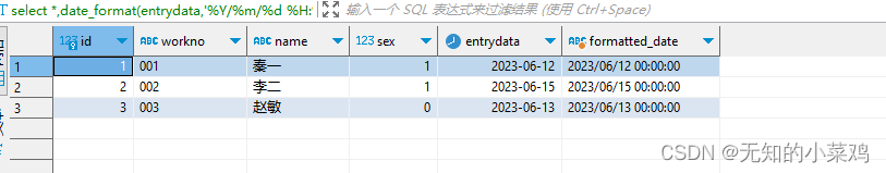
三个主流数据库(Oracle、MySQL和SQL Server)的“单表造数
oracle 1.创建表 CREATE TABLE "YZH2_ORACLE" ("VARCHAR2_COLUMN" VARCHAR2(20) NOT NULL ENABLE,"NUMBER_COLUMN" NUMBER,"DATE_COLUMN" DATE,"CLOB_COLUMN" CLOB,"BLOB_COLUMN" BLOB,"BINARY_DOUBLE_COLU…...

TypeScript 中【class类】与 【 接口 Interfaces】的联合搭配使用解读
导读: 前面章节,我们讲到过 接口(Interface)可以用于对「对象的形状(Shape)」进行描述。 本章节主要介绍接口的另一个用途,对类的一部分行为进行抽象。 类配合实现接口 实现(impleme…...
JavaWeb 手写Tomcat底层机制
目录 一、Tomcat底层整体架构 1.简介 : 2.分析图 : 3.基于Socket开发服务端的流程 : 4.打通服务器端和客户端的数据通道 : 二、多线程模型的实现 1.思路分析 : 2.处理HTTP请求 : 3.自定义Tomcat : 三、自定义Servlet规范 1. HTTP请求和响应 : 1 CyanServletRequest …...
Gof23设计模式之组合模式
1.定义 组合模式又名部分整体模式,是用于把一组相似的对象当作一个单一的对象。组合模式依据树形结构来组合对象,用来表示部分以及整体层次。这种类型的设计模式属于结构型模式,它创建了对象组的树形结构。 2.结构 组合模式主要包含三种…...
龙芯积极研发二进制翻译,提升软硬件兼容性,提高LoongArch架构
根据8月8日Phoronix报道,龙芯正在积极研发龙芯二进制翻译功能(Loongson Binary Translationm,LBT)以提高LoongArch架构与其他处理器(如MIPS/x86/Arm)的二进制翻译能力,这重要举措将显著提升龙芯…...

3天爆肝整理,自动化测试-YAML文件读写实战(超细总结)
目录:导读 前言一、Python编程入门到精通二、接口自动化项目实战三、Web自动化项目实战四、App自动化项目实战五、一线大厂简历六、测试开发DevOps体系七、常用自动化测试工具八、JMeter性能测试九、总结(尾部小惊喜) 前言 YAML 简介 YAML&…...

算法通关村——透彻理解二分查找
1. 循环法 public static int binarySearch(int[] arr, int low, int high, int target) {while (low < high) {// 这样写主要是避免溢出的情况,以及>>优先级小于,避免出现死循环int mid low ((high - low) >> 1);if (arr[mid] target…...
刷题指南 —— 第六弹(⭐有点难度⭐))
PAT(Advanced Level)刷题指南 —— 第六弹(⭐有点难度⭐)
一、1010 Radix 1. 问题重述 2. Sample Input1 6 110 1 103. Sample Output1 24. Sample Input 2 1 ab 1 25. Sample Output 2...

个人对智能家居平台选择的思考
本人之前开发过不少MicroPython程序,其中涉及到自动化以及局域网控制思路,也可以作为智能家居的实现方式。而NodeMCUESPHome的方案具有方便添加硬件、容易更新程序和容量占用小的优势,本人也查看过相关教程后感觉部署ESPHome和编译固件的步骤…...

无涯教程-Lua - while语句函数
只要给定条件为真,Lua编程语言中的 while 循环语句就会重复执行目标语句。 while loop - 语法 Lua编程语言中 while 循环的语法如下- while(condition) dostatement(s) end while loop - 流程图 在这里,需要注意的关键是 while 循环可能根本不执行。…...
MySql学习3:常用函数
常用字符串函数 CHAR_LENGTH(s):返回字符串的长度 select *, char_length(name) as nameLength from emp;CONCAT(s1,s2…sn):字符串拼接 select name,concat(name,入职时间:,entrydata) as 入职时间 from emp;CONCAT_WS(x, s1,s2…sn)&a…...

24届近5年江南大学自动化考研院校分析
今天给大家带来的是江南大学控制考研分析 满满干货~还不快快点赞收藏 一、江南大学 学校简介 江南大学(Jiangnan University)是国家“双一流”建设高校,“211工程”、“985工程优势学科创新平台”重点建设高校,入选…...
C++ 数组
数组是具有一定顺序关系的若干对象的集合体,组成数组的对象称为该数组的元素。 数组元素用数组名与带方括号的下标表示,同一数组的各个元素具有相同的类型。数组可以由除void型以外的任何一种类型构成,构成数组的类型和数组之间的关系&#x…...
Android LinearLayout dynamic add child ImageView,Glide load,kotlin
Android LinearLayout dynamic add child ImageView,Glide load,kotlin images.xml <?xml version"1.0" encoding"utf-8"?> <LinearLayout xmlns:android"http://schemas.android.com/apk/res/android"andro…...

Android Wi-Fi 连接失败日志分析
1. Android wifi 关键日志总结 (1) Wi-Fi 断开 (CTRL-EVENT-DISCONNECTED reason3) 日志相关部分: 06-05 10:48:40.987 943 943 I wpa_supplicant: wlan0: CTRL-EVENT-DISCONNECTED bssid44:9b:c1:57:a8:90 reason3 locally_generated1解析: CTR…...

DeepSeek 赋能智慧能源:微电网优化调度的智能革新路径
目录 一、智慧能源微电网优化调度概述1.1 智慧能源微电网概念1.2 优化调度的重要性1.3 目前面临的挑战 二、DeepSeek 技术探秘2.1 DeepSeek 技术原理2.2 DeepSeek 独特优势2.3 DeepSeek 在 AI 领域地位 三、DeepSeek 在微电网优化调度中的应用剖析3.1 数据处理与分析3.2 预测与…...

逻辑回归:给不确定性划界的分类大师
想象你是一名医生。面对患者的检查报告(肿瘤大小、血液指标),你需要做出一个**决定性判断**:恶性还是良性?这种“非黑即白”的抉择,正是**逻辑回归(Logistic Regression)** 的战场&a…...
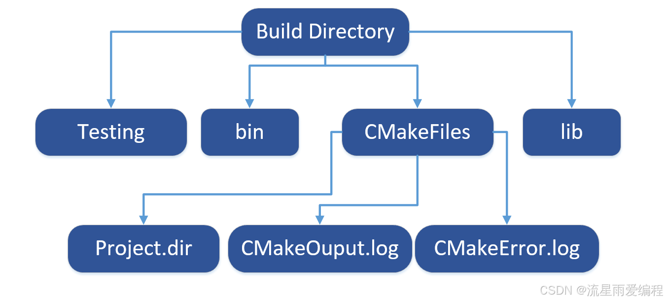
CMake基础:构建流程详解
目录 1.CMake构建过程的基本流程 2.CMake构建的具体步骤 2.1.创建构建目录 2.2.使用 CMake 生成构建文件 2.3.编译和构建 2.4.清理构建文件 2.5.重新配置和构建 3.跨平台构建示例 4.工具链与交叉编译 5.CMake构建后的项目结构解析 5.1.CMake构建后的目录结构 5.2.构…...

基于数字孪生的水厂可视化平台建设:架构与实践
分享大纲: 1、数字孪生水厂可视化平台建设背景 2、数字孪生水厂可视化平台建设架构 3、数字孪生水厂可视化平台建设成效 近几年,数字孪生水厂的建设开展的如火如荼。作为提升水厂管理效率、优化资源的调度手段,基于数字孪生的水厂可视化平台的…...

AI病理诊断七剑下天山,医疗未来触手可及
一、病理诊断困局:刀尖上的医学艺术 1.1 金标准背后的隐痛 病理诊断被誉为"诊断的诊断",医生需通过显微镜观察组织切片,在细胞迷宫中捕捉癌变信号。某省病理质控报告显示,基层医院误诊率达12%-15%,专家会诊…...
免费PDF转图片工具
免费PDF转图片工具 一款简单易用的PDF转图片工具,可以将PDF文件快速转换为高质量PNG图片。无需安装复杂的软件,也不需要在线上传文件,保护您的隐私。 工具截图 主要特点 🚀 快速转换:本地转换,无需等待上…...

基于Springboot+Vue的办公管理系统
角色: 管理员、员工 技术: 后端: SpringBoot, Vue2, MySQL, Mybatis-Plus 前端: Vue2, Element-UI, Axios, Echarts, Vue-Router 核心功能: 该办公管理系统是一个综合性的企业内部管理平台,旨在提升企业运营效率和员工管理水…...

人工智能--安全大模型训练计划:基于Fine-tuning + LLM Agent
安全大模型训练计划:基于Fine-tuning LLM Agent 1. 构建高质量安全数据集 目标:为安全大模型创建高质量、去偏、符合伦理的训练数据集,涵盖安全相关任务(如有害内容检测、隐私保护、道德推理等)。 1.1 数据收集 描…...

土建施工员考试:建筑施工技术重点知识有哪些?
《管理实务》是土建施工员考试中侧重实操应用与管理能力的科目,核心考查施工组织、质量安全、进度成本等现场管理要点。以下是结合考试大纲与高频考点整理的重点内容,附学习方向和应试技巧: 一、施工组织与进度管理 核心目标: 规…...