【Python机器学习】实验15 将Lenet5应用于Cifar10数据集(PyTorch实现)
文章目录
- CIFAR10数据集介绍
- 1. 数据的下载
- 2.修改模型与前面的参数设置保持一致
- 3. 新建模型
- 4. 从数据集中分批量读取数据
- 5. 定义损失函数
- 6. 定义优化器
- 7. 开始训练
- 8.测试模型
- 9. 手写体图片的可视化
- 10. 多幅图片的可视化
- 思考题
- 11. 读取测试集的图片预测值(神经网络的输出为10)
- 12. 采用pandas可视化数据
- 13. 对预测错误的样本点进行可视化
- 14. 看看错误样本被预测为哪些数据?
- 15.输出错误的模型类别
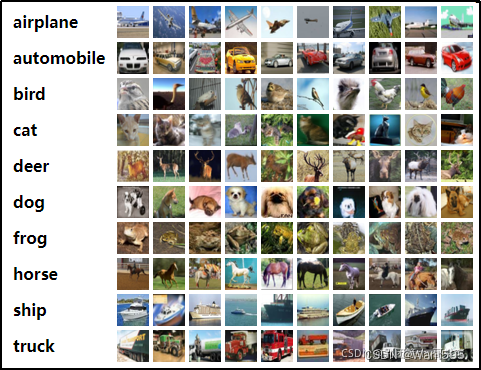
CIFAR10数据集介绍
CIFAR-10 数据集由10个类别的60000张32x32彩色图像组成,每类6000张图像。有50000张训练图像和10000张测试图像。数据集分为五个训练批次
和一个测试批次,每个批次有10000张图像。测试批次包含从每个类别中随机选择的1000张图像。训练批次包含随机顺序的剩余图像,但一些训练批次
可能包含比另一个类别更多的图像。在它们之间训练批次包含来自每个类的5000张图像。以下是数据集中的类,以及每个类中的10张随机图像:
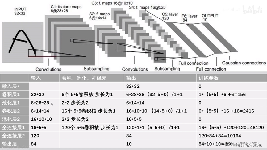
因为CIFAR10数据集颜色通道有3个,所以卷积层L1的输入通道数量(in_channels)需要设为3。全连接层fc1的输入维度设为400,这与上例设为256有所不同,原因是初始输入数据的形状不一样,经过卷积池化后,输出的数据形状是不一样的。如果是采用动态图开发模型,那么有一种便捷的方式查看中间结果的形状,即在forward()方法中,用print函数把中间结果的形状打印出来。根据中间结果的形状,决定接下来各网络层的参数。
1. 数据的下载
import torch
import torchvision.transforms as transforms
from torchvision.datasets import CIFAR10
train_dataset = CIFAR10(root="./data/CIFAR10",train=True,transform=transforms.ToTensor(),download=True)
test_dataset = CIFAR10(root="./data/CIFAR10", train=False,transform=transforms.ToTensor())
Files already downloaded and verified
train_dataset[0][0].shape
torch.Size([3, 32, 32])
train_dataset[0][1]
6
2.修改模型与前面的参数设置保持一致
from torch import nn
class Lenet5(nn.Module):def __init__(self):super(Lenet5,self).__init__()#1+ 32-5/(1)==28self.features=nn.Sequential(#定义第一个卷积层nn.Conv2d(in_channels=3,out_channels=6,kernel_size=(5,5),stride=1),nn.ReLU(),nn.AvgPool2d(kernel_size=2,stride=2),#定义第二个卷积层nn.Conv2d(in_channels=6,out_channels=16,kernel_size=(5,5),stride=1),nn.ReLU(),nn.MaxPool2d(kernel_size=2,stride=2),)#定义全连接层self.classfier=nn.Sequential(nn.Linear(in_features=400,out_features=120),nn.ReLU(),nn.Linear(in_features=120,out_features=84),nn.ReLU(),nn.Linear(in_features=84,out_features=10), )def forward(self,x):x=self.features(x)x=torch.flatten(x,1)result=self.classfier(x)return result
3. 新建模型
model=Lenet5()
device=torch.device("cuda:0" if torch.cuda.is_available() else "cpu")
model=model.to(device)
4. 从数据集中分批量读取数据
#加载数据集
batch_size=32
train_loader= torch.utils.data.DataLoader(train_dataset, batch_size, shuffle=True)
test_loader= torch.utils.data.DataLoader(test_dataset, batch_size, shuffle=False)
# 类别信息也是需要我们给定的
classes = ('plane', 'car', 'bird', 'cat','deer', 'dog', 'frog', 'horse', 'ship', 'truck')
5. 定义损失函数
from torch import optim
loss_fun=nn.CrossEntropyLoss()
loss_lst=[]
6. 定义优化器
optimizer=optim.SGD(params=model.parameters(),lr=0.001,momentum=0.9)
7. 开始训练
import time
start_time=time.time()
#训练的迭代次数
for epoch in range(10):loss_i=0for i,(batch_data,batch_label) in enumerate(train_loader):#清空优化器的梯度optimizer.zero_grad()#模型前向预测pred=model(batch_data)loss=loss_fun(pred,batch_label)loss_i+=lossloss.backward()optimizer.step()if (i+1)%200==0:print("第%d次训练,第%d批次,损失为%.2f"%(epoch,i,loss_i/200))loss_i=0
end_time=time.time()
print("共训练了%d 秒"%(end_time-start_time))
第0次训练,第199批次,损失为2.30
第0次训练,第399批次,损失为2.30
第0次训练,第599批次,损失为2.30
第0次训练,第799批次,损失为2.30
第0次训练,第999批次,损失为2.30
第0次训练,第1199批次,损失为2.30
第0次训练,第1399批次,损失为2.30
第1次训练,第199批次,损失为2.30
第1次训练,第399批次,损失为2.30
第1次训练,第599批次,损失为2.30
第1次训练,第799批次,损失为2.30
第1次训练,第999批次,损失为2.29
第1次训练,第1199批次,损失为2.27
第1次训练,第1399批次,损失为2.18
第2次训练,第199批次,损失为2.07
第2次训练,第399批次,损失为2.04
第2次训练,第599批次,损失为2.03
第2次训练,第799批次,损失为2.00
第2次训练,第999批次,损失为1.98
第2次训练,第1199批次,损失为1.96
第2次训练,第1399批次,损失为1.95
第3次训练,第199批次,损失为1.89
第3次训练,第399批次,损失为1.86
第3次训练,第599批次,损失为1.84
第3次训练,第799批次,损失为1.80
第3次训练,第999批次,损失为1.75
第3次训练,第1199批次,损失为1.71
第3次训练,第1399批次,损失为1.71
第4次训练,第199批次,损失为1.66
第4次训练,第399批次,损失为1.65
第4次训练,第599批次,损失为1.63
第4次训练,第799批次,损失为1.61
第4次训练,第999批次,损失为1.62
第4次训练,第1199批次,损失为1.60
第4次训练,第1399批次,损失为1.59
第5次训练,第199批次,损失为1.56
第5次训练,第399批次,损失为1.56
第5次训练,第599批次,损失为1.54
第5次训练,第799批次,损失为1.55
第5次训练,第999批次,损失为1.52
第5次训练,第1199批次,损失为1.52
第5次训练,第1399批次,损失为1.49
第6次训练,第199批次,损失为1.50
第6次训练,第399批次,损失为1.47
第6次训练,第599批次,损失为1.46
第6次训练,第799批次,损失为1.47
第6次训练,第999批次,损失为1.46
第6次训练,第1199批次,损失为1.43
第6次训练,第1399批次,损失为1.45
第7次训练,第199批次,损失为1.42
第7次训练,第399批次,损失为1.42
第7次训练,第599批次,损失为1.39
第7次训练,第799批次,损失为1.39
第7次训练,第999批次,损失为1.40
第7次训练,第1199批次,损失为1.40
第7次训练,第1399批次,损失为1.40
第8次训练,第199批次,损失为1.36
第8次训练,第399批次,损失为1.37
第8次训练,第599批次,损失为1.38
第8次训练,第799批次,损失为1.37
第8次训练,第999批次,损失为1.34
第8次训练,第1199批次,损失为1.37
第8次训练,第1399批次,损失为1.35
第9次训练,第199批次,损失为1.31
第9次训练,第399批次,损失为1.31
第9次训练,第599批次,损失为1.31
第9次训练,第799批次,损失为1.31
第9次训练,第999批次,损失为1.34
第9次训练,第1199批次,损失为1.32
第9次训练,第1399批次,损失为1.31
共训练了156 秒
8.测试模型
len(test_dataset)
10000
correct=0
for batch_data,batch_label in test_loader:pred_test=model(batch_data)pred_result=torch.max(pred_test.data,1)[1]correct+=(pred_result==batch_label).sum()
print("准确率为:%.2f%%"%(correct/len(test_dataset)))
准确率为:0.53%
9. 手写体图片的可视化
from torchvision import transforms as T
import torch
len(train_dataset)
50000
train_dataset[0][0].shape
torch.Size([3, 32, 32])
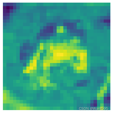
import matplotlib.pyplot as plt
plt.imshow(train_dataset[0][0][0],cmap="gray")
plt.axis('off')
(-0.5, 31.5, 31.5, -0.5)

plt.imshow(train_dataset[0][0][0])
plt.axis('off')
(-0.5, 31.5, 31.5, -0.5)
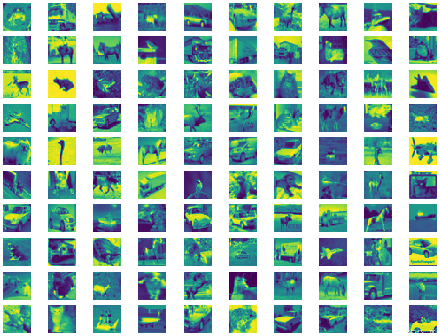
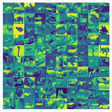
10. 多幅图片的可视化
from matplotlib import pyplot as plt
plt.figure(figsize=(20,15))
cols=10
rows=10
for i in range(0,rows):for j in range(0,cols):idx=j+i*colsplt.subplot(rows,cols,idx+1) plt.imshow(train_dataset[idx][0][0])plt.axis('off')
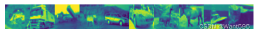
import numpy as np
img10 = np.stack(list(train_dataset[i][0][0] for i in range(10)), axis=1).reshape(32,320)
plt.imshow(img10)
plt.axis('off')
(-0.5, 319.5, 31.5, -0.5)
img100 = np.stack( tuple( np.stack(tuple( train_dataset[j*10+i][0][0] for i in range(10) ), axis=1).reshape(32,320) for j in range(10)),axis=0).reshape(320,320)
plt.imshow(img100)
plt.axis('off')
(-0.5, 319.5, 319.5, -0.5)
思考题
- 测试集中有哪些识别错误的手写数字图片? 汇集整理并分析原因?
11. 读取测试集的图片预测值(神经网络的输出为10)
pre_result=torch.zeros(len(test_dataset),10)
for i in range(len(test_dataset)):pre_result[i,:]=model(torch.reshape(test_dataset[i][0],(-1,3,32,32)))
pre_result
tensor([[-0.4934, -1.0982, 0.4072, ..., -0.4038, -1.1655, -0.8201],[ 4.0154, 4.4736, -0.2921, ..., -2.3925, 4.3176, 4.1910],[ 1.3858, 3.2022, -0.7004, ..., -2.2767, 3.0923, 2.3740],...,[-1.9551, -3.8085, 1.7917, ..., 2.1104, -2.9573, -1.7387],[ 0.6681, -0.5328, 0.3059, ..., 0.1170, -2.5236, -0.5746],[-0.5194, -2.6185, 1.1929, ..., 3.7749, -2.3134, -1.5123]],grad_fn=<CopySlices>)
pre_result.shape
torch.Size([10000, 10])
pre_result[:5]
tensor([[-0.4934, -1.0982, 0.4072, 1.7331, -0.4456, 1.6433, 0.1721, -0.4038,-1.1655, -0.8201],[ 4.0154, 4.4736, -0.2921, -3.2882, -1.6234, -4.4814, -3.1241, -2.3925,4.3176, 4.1910],[ 1.3858, 3.2022, -0.7004, -1.0123, -1.7394, -1.6657, -3.2578, -2.2767,3.0923, 2.3740],[ 2.1151, 0.8262, 0.0071, -1.1410, -0.3051, -2.0239, -2.3023, -0.3573,2.9400, 0.5595],[-2.3524, -2.7907, 1.9834, 2.1088, 2.7645, 1.1118, 2.9782, -0.3876,-3.2325, -2.3916]], grad_fn=<SliceBackward0>)
#显示这10000张图片的标签
label_10000=[test_dataset[i][1] for i in range(10000)]
label_10000
[3,8,8,0,6,6,1,6,3,1,0,9,5,7,9,8,5,7,8,6,7,0,4,9,5,2,4,0,9,6,6,5,4,5,9,2,4,1,9,5,4,6,5,6,0,9,3,9,7,6,9,8,0,3,8,8,7,7,4,6,7,3,6,3,6,2,1,2,3,7,2,6,8,8,0,2,9,3,3,8,8,1,1,7,2,5,2,7,8,9,0,3,8,6,4,6,6,0,0,7,4,5,6,3,1,1,3,6,8,7,4,0,6,2,1,3,0,4,2,7,8,3,1,2,8,0,8,3,5,2,4,1,8,9,1,2,9,7,2,9,6,5,6,3,8,7,6,2,5,2,8,9,6,0,0,5,2,9,5,4,2,1,6,6,8,4,8,4,5,0,9,9,9,8,9,9,3,7,5,0,0,5,2,2,3,8,6,3,4,0,5,8,0,1,7,2,8,8,7,8,5,1,8,7,1,3,0,5,7,9,7,4,5,9,8,0,7,9,8,2,7,6,9,4,3,9,6,4,7,6,5,1,5,8,8,0,4,0,5,5,1,1,8,9,0,3,1,9,2,2,5,3,9,9,4,0,3,0,0,9,8,1,5,7,0,8,2,4,7,0,2,3,6,3,8,5,0,3,4,3,9,0,6,1,0,9,1,0,7,9,1,2,6,9,3,4,6,0,0,6,6,6,3,2,6,1,8,2,1,6,8,6,8,0,4,0,7,7,5,5,3,5,2,3,4,1,7,5,4,6,1,9,3,6,6,9,3,8,0,7,2,6,2,5,8,5,4,6,8,9,9,1,0,2,2,7,3,2,8,0,9,5,8,1,9,4,1,3,8,1,4,7,9,4,2,7,0,7,0,6,6,9,0,9,2,8,7,2,2,5,1,2,6,2,9,6,2,3,0,3,9,8,7,8,8,4,0,1,8,2,7,9,3,6,1,9,0,7,3,7,4,5,0,0,2,9,3,4,0,6,2,5,3,7,3,7,2,5,3,1,1,4,9,9,5,7,5,0,2,2,2,9,7,3,9,4,3,5,4,6,5,6,1,4,3,4,4,3,7,8,3,7,8,0,5,7,6,0,5,4,8,6,8,5,5,9,9,9,5,0,1,0,8,1,1,8,0,2,2,0,4,6,5,4,9,4,7,9,9,4,5,6,6,1,5,3,8,9,5,8,5,7,0,7,0,5,0,0,4,6,9,0,9,5,6,6,6,2,9,0,1,7,6,7,5,9,1,6,2,5,5,5,8,5,9,4,6,4,3,2,0,7,6,2,2,3,9,7,9,2,6,7,1,3,6,6,8,9,7,5,4,0,8,4,0,9,3,4,8,9,6,9,2,6,1,4,7,3,5,3,8,5,0,2,1,6,4,3,3,9,6,9,8,8,5,8,6,6,2,1,7,7,1,2,7,9,9,4,4,1,2,5,6,8,7,6,8,3,0,5,5,3,0,7,9,1,3,4,4,5,3,9,5,6,9,2,1,1,4,1,9,4,7,6,3,8,9,0,1,3,6,3,6,3,2,0,3,1,0,5,9,6,4,8,9,6,9,6,3,0,3,2,2,7,8,3,8,2,7,5,7,2,4,8,7,4,2,9,8,8,6,8,8,7,4,3,3,8,4,9,4,8,8,1,8,2,1,3,6,5,4,2,7,9,9,4,1,4,1,3,2,7,0,7,9,7,6,6,2,5,9,2,9,1,2,2,6,8,2,1,3,6,6,0,1,2,7,0,5,4,6,1,6,4,0,2,2,6,0,5,9,1,7,6,7,0,3,9,6,8,3,0,3,4,7,7,1,4,7,2,7,1,4,7,4,4,8,4,7,7,5,3,7,2,0,8,9,5,8,3,6,2,0,8,7,3,7,6,5,3,1,3,2,2,5,4,1,2,9,2,7,0,7,2,1,3,2,0,2,4,7,9,8,9,0,7,7,0,7,8,4,6,3,3,0,1,3,7,0,1,3,1,4,2,3,8,4,2,3,7,8,4,3,0,9,0,0,1,0,4,4,6,7,6,1,1,3,7,3,5,2,6,6,5,8,7,1,6,8,8,5,3,0,4,0,1,3,8,8,0,6,9,9,9,5,5,8,6,0,0,4,2,3,2,7,2,2,5,9,8,9,1,7,4,0,3,0,1,3,8,3,9,6,1,4,7,0,3,7,8,9,1,1,6,6,6,6,9,1,9,9,4,2,1,7,0,6,8,1,9,2,9,0,4,7,8,3,1,2,0,1,5,8,4,6,3,8,1,3,8,...]
import numpy
pre_10000=pre_result.detach()
pre_10000
tensor([[-0.4934, -1.0982, 0.4072, ..., -0.4038, -1.1655, -0.8201],[ 4.0154, 4.4736, -0.2921, ..., -2.3925, 4.3176, 4.1910],[ 1.3858, 3.2022, -0.7004, ..., -2.2767, 3.0923, 2.3740],...,[-1.9551, -3.8085, 1.7917, ..., 2.1104, -2.9573, -1.7387],[ 0.6681, -0.5328, 0.3059, ..., 0.1170, -2.5236, -0.5746],[-0.5194, -2.6185, 1.1929, ..., 3.7749, -2.3134, -1.5123]])
pre_10000=numpy.array(pre_10000)
pre_10000
array([[-0.49338394, -1.098238 , 0.40724754, ..., -0.40375623,-1.165497 , -0.820113 ],[ 4.0153656 , 4.4736323 , -0.29209492, ..., -2.392501 ,4.317573 , 4.190993 ],[ 1.3858219 , 3.2021556 , -0.70040375, ..., -2.2767155 ,3.092283 , 2.373978 ],...,[-1.9550545 , -3.808494 , 1.7917161 , ..., 2.110389 ,-2.9572597 , -1.7386926 ],[ 0.66809845, -0.5327946 , 0.30590305, ..., 0.11701592,-2.5236375 , -0.5746133 ],[-0.51935434, -2.6184506 , 1.1929085 , ..., 3.7748828 ,-2.3134274 , -1.5123445 ]], dtype=float32)
12. 采用pandas可视化数据
import pandas as pd
table=pd.DataFrame(zip(pre_10000,label_10000))
table
| 0 | 1 | |
|---|---|---|
| 0 | [-0.49338394, -1.098238, 0.40724754, 1.7330961... | 3 |
| 1 | [4.0153656, 4.4736323, -0.29209492, -3.2882178... | 8 |
| 2 | [1.3858219, 3.2021556, -0.70040375, -1.0123051... | 8 |
| 3 | [2.11508, 0.82618773, 0.007076204, -1.1409527,... | 0 |
| 4 | [-2.352432, -2.7906854, 1.9833877, 2.1087575, ... | 6 |
| ... | ... | ... |
| 9995 | [-0.55809855, -4.3891077, -0.3040389, 3.001731... | 8 |
| 9996 | [-2.7151718, -4.1596007, 1.2393914, 2.8491826,... | 3 |
| 9997 | [-1.9550545, -3.808494, 1.7917161, 2.6365147, ... | 5 |
| 9998 | [0.66809845, -0.5327946, 0.30590305, -0.182045... | 1 |
| 9999 | [-0.51935434, -2.6184506, 1.1929085, 0.1288419... | 7 |
10000 rows × 2 columns
table[0].values
array([array([-0.49338394, -1.098238 , 0.40724754, 1.7330961 , -0.4455951 ,1.6433077 , 0.1720748 , -0.40375623, -1.165497 , -0.820113 ],dtype=float32) ,array([ 4.0153656 , 4.4736323 , -0.29209492, -3.2882178 , -1.6234205 ,-4.481386 , -3.1240807 , -2.392501 , 4.317573 , 4.190993 ],dtype=float32) ,array([ 1.3858219 , 3.2021556 , -0.70040375, -1.0123051 , -1.7393746 ,-1.6656632 , -3.2578242 , -2.2767155 , 3.092283 , 2.373978 ],dtype=float32) ,...,array([-1.9550545 , -3.808494 , 1.7917161 , 2.6365147 , 0.37311587,3.545672 , -0.43889195, 2.110389 , -2.9572597 , -1.7386926 ],dtype=float32) ,array([ 0.66809845, -0.5327946 , 0.30590305, -0.18204585, 2.0045712 ,0.47369143, -0.3122899 , 0.11701592, -2.5236375 , -0.5746133 ],dtype=float32) ,array([-0.51935434, -2.6184506 , 1.1929085 , 0.1288419 , 1.8770852 ,0.4296908 , -0.22015049, 3.7748828 , -2.3134274 , -1.5123445 ],dtype=float32) ],dtype=object)
table["pred"]=[np.argmax(table[0][i]) for i in range(table.shape[0])]
table
| 0 | 1 | pred | |
|---|---|---|---|
| 0 | [-0.49338394, -1.098238, 0.40724754, 1.7330961... | 3 | 3 |
| 1 | [4.0153656, 4.4736323, -0.29209492, -3.2882178... | 8 | 1 |
| 2 | [1.3858219, 3.2021556, -0.70040375, -1.0123051... | 8 | 1 |
| 3 | [2.11508, 0.82618773, 0.007076204, -1.1409527,... | 0 | 8 |
| 4 | [-2.352432, -2.7906854, 1.9833877, 2.1087575, ... | 6 | 6 |
| ... | ... | ... | ... |
| 9995 | [-0.55809855, -4.3891077, -0.3040389, 3.001731... | 8 | 5 |
| 9996 | [-2.7151718, -4.1596007, 1.2393914, 2.8491826,... | 3 | 3 |
| 9997 | [-1.9550545, -3.808494, 1.7917161, 2.6365147, ... | 5 | 5 |
| 9998 | [0.66809845, -0.5327946, 0.30590305, -0.182045... | 1 | 4 |
| 9999 | [-0.51935434, -2.6184506, 1.1929085, 0.1288419... | 7 | 7 |
10000 rows × 3 columns
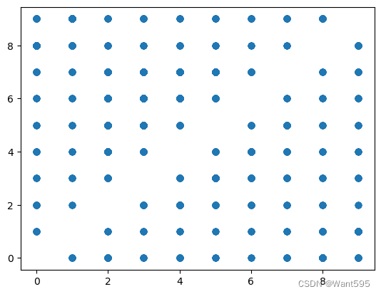
13. 对预测错误的样本点进行可视化
mismatch=table[table[1]!=table["pred"]]
mismatch
| 0 | 1 | pred | |
|---|---|---|---|
| 1 | [4.0153656, 4.4736323, -0.29209492, -3.2882178... | 8 | 1 |
| 2 | [1.3858219, 3.2021556, -0.70040375, -1.0123051... | 8 | 1 |
| 3 | [2.11508, 0.82618773, 0.007076204, -1.1409527,... | 0 | 8 |
| 8 | [0.02641207, -3.6653092, 2.294829, 2.2884543, ... | 3 | 5 |
| 12 | [-1.4556388, -1.7955011, -0.6100754, 1.169481,... | 5 | 6 |
| ... | ... | ... | ... |
| 9989 | [-0.2553262, -2.8777533, 3.4579017, 0.3079242,... | 2 | 4 |
| 9993 | [-0.077826336, -3.14616, 0.8994149, 3.5604722,... | 5 | 3 |
| 9994 | [-1.2543154, -2.4472265, 0.6754027, 2.0582433,... | 3 | 6 |
| 9995 | [-0.55809855, -4.3891077, -0.3040389, 3.001731... | 8 | 5 |
| 9998 | [0.66809845, -0.5327946, 0.30590305, -0.182045... | 1 | 4 |
4657 rows × 3 columns
from matplotlib import pyplot as plt
plt.scatter(mismatch[1],mismatch["pred"])
<matplotlib.collections.PathCollection at 0x1b3a92ef910>
14. 看看错误样本被预测为哪些数据?
mismatch[mismatch[1]==9].sort_values("pred").index
Int64Index([2129, 1465, 2907, 787, 2902, 2307, 4588, 5737, 8276, 8225,...7635, 7553, 7526, 3999, 1626, 1639, 4193, 7198, 3957, 3344],dtype='int64', length=396)
idx_lst=mismatch[mismatch[1]==9].sort_values("pred").index.values
idx_lst,len(idx_lst)
(array([2129, 1465, 2907, 787, 2902, 2307, 4588, 5737, 8276, 8225, 8148,4836, 1155, 7218, 8034, 7412, 5069, 1629, 5094, 5109, 7685, 5397,1427, 5308, 8727, 2960, 2491, 6795, 1997, 6686, 9449, 6545, 8985,9401, 3564, 6034, 383, 9583, 9673, 507, 3288, 6868, 9133, 9085,577, 4261, 6974, 411, 6290, 5416, 5350, 5950, 5455, 5498, 6143,5964, 5864, 5877, 6188, 5939, 14, 5300, 3501, 3676, 3770, 3800,3850, 3893, 3902, 4233, 4252, 4253, 4276, 5335, 4297, 4418, 4445,4536, 4681, 6381, 4929, 4945, 5067, 5087, 5166, 5192, 4364, 4928,7024, 6542, 8144, 8312, 8385, 8406, 8453, 8465, 8521, 8585, 8673,8763, 8946, 9067, 9069, 9199, 9209, 9217, 9280, 9403, 9463, 9518,9692, 9743, 9871, 9875, 9881, 8066, 6509, 8057, 7826, 6741, 6811,6814, 6840, 6983, 7007, 3492, 7028, 7075, 7121, 7232, 7270, 7424,7431, 7444, 7492, 7499, 7501, 7578, 7639, 7729, 7767, 7792, 7818,7824, 7942, 3459, 4872, 1834, 1487, 1668, 1727, 1732, 1734, 1808,1814, 1815, 1831, 1927, 2111, 2126, 2190, 2246, 2290, 2433, 2596,2700, 2714, 1439, 1424, 1376, 1359, 28, 151, 172, 253, 259,335, 350, 591, 625, 2754, 734, 940, 951, 970, 1066, 1136,1177, 1199, 1222, 1231, 853, 2789, 9958, 2946, 3314, 3307, 2876,3208, 3166, 2944, 2817, 2305, 7522, 7155, 7220, 4590, 2899, 2446,2186, 7799, 9492, 3163, 4449, 2027, 2387, 1064, 3557, 2177, 654,9791, 2670, 2514, 2495, 3450, 8972, 3210, 3755, 2756, 7967, 3970,4550, 6017, 938, 744, 6951, 3397, 4852, 3133, 7931, 707, 3312,7470, 6871, 8292, 7100, 9529, 9100, 3853, 9060, 9732, 2521, 3789,2974, 5311, 3218, 5736, 3055, 7076, 1220, 9147, 1344, 532, 8218,3569, 1008, 8475, 8877, 1582, 8936, 4758, 1837, 9517, 252, 5832,1916, 6369, 4979, 9324, 6218, 9777, 7923, 4521, 2868, 213, 8083,5952, 5579, 4508, 5488, 2460, 5332, 5180, 8323, 8345, 3776, 2568,5151, 4570, 2854, 8488, 4874, 680, 2810, 1285, 6136, 3339, 9143,6852, 1906, 7067, 7073, 2975, 1924, 6804, 6755, 9299, 2019, 9445,9560, 360, 1601, 7297, 9122, 6377, 9214, 6167, 3980, 394, 7491,7581, 9349, 8953, 222, 139, 530, 3577, 9868, 247, 9099, 9026,209, 538, 3229, 9258, 585, 9204, 9643, 1492, 3609, 6570, 6561,6469, 6435, 6419, 2155, 6275, 4481, 2202, 1987, 2271, 2355, 2366,2432, 5400, 2497, 2727, 4931, 4619, 9884, 5902, 8796, 6848, 6960,8575, 8413, 981, 8272, 8145, 3172, 1221, 3168, 1256, 1889, 1291,3964, 7635, 7553, 7526, 3999, 1626, 1639, 4193, 7198, 3957, 3344],dtype=int64),396)
import numpy as np
img=np.stack(list(test_dataset[idx_lst[i]][0][0] for i in range(5)),axis=1).reshape(32,32*5)
plt.imshow(img)
plt.axis('off')
(-0.5, 159.5, 31.5, -0.5)
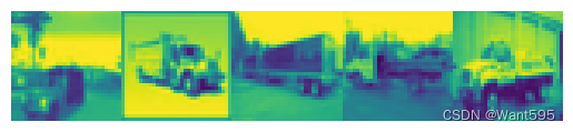
#显示4行
import numpy as np
img20=np.stack(tuple(np.stack(tuple(test_dataset[idx_lst[i+j*5]][0][0] for i in range(5)),axis=1).reshape(32,32*5) for j in range(4)),axis=0).reshape(32*4,32*5)
plt.imshow(img20)
plt.axis('off')
(-0.5, 159.5, 127.5, -0.5)

15.输出错误的模型类别
idx_lst=mismatch[mismatch[1]==9].index.values
table.iloc[idx_lst[:], 2].values
array([1, 1, 8, 1, 1, 8, 7, 8, 8, 6, 1, 1, 1, 1, 7, 0, 7, 0, 0, 8, 6, 8,0, 8, 1, 1, 3, 7, 5, 1, 4, 0, 1, 4, 1, 1, 1, 8, 6, 3, 1, 1, 0, 1,1, 6, 8, 1, 1, 8, 7, 8, 6, 1, 1, 1, 0, 1, 0, 1, 8, 6, 7, 8, 0, 8,1, 1, 1, 1, 1, 1, 1, 1, 1, 6, 8, 7, 6, 7, 1, 8, 0, 7, 3, 1, 1, 0,8, 3, 3, 1, 8, 1, 8, 1, 2, 0, 8, 8, 3, 8, 1, 3, 7, 0, 3, 8, 3, 5,7, 1, 3, 1, 1, 8, 1, 3, 1, 7, 1, 7, 7, 1, 3, 0, 0, 1, 1, 0, 5, 7,6, 4, 3, 1, 8, 8, 1, 3, 5, 8, 0, 1, 5, 1, 7, 8, 4, 3, 1, 1, 1, 3,0, 6, 8, 8, 1, 3, 1, 7, 5, 1, 1, 5, 1, 1, 8, 8, 4, 7, 8, 8, 1, 1,1, 0, 1, 1, 1, 1, 1, 3, 8, 7, 7, 1, 4, 7, 0, 2, 8, 1, 6, 0, 4, 1,7, 1, 1, 8, 1, 6, 1, 0, 1, 0, 0, 7, 1, 7, 1, 1, 0, 5, 7, 1, 1, 0,8, 1, 1, 7, 1, 7, 5, 0, 6, 1, 1, 8, 1, 1, 7, 1, 4, 0, 7, 1, 7, 1,6, 8, 1, 6, 7, 1, 8, 8, 8, 1, 1, 0, 8, 8, 0, 1, 7, 0, 7, 1, 1, 1,8, 7, 0, 5, 4, 8, 0, 1, 1, 1, 1, 7, 7, 1, 6, 5, 1, 2, 8, 0, 2, 1,1, 7, 0, 1, 1, 1, 5, 7, 1, 1, 1, 2, 8, 8, 1, 7, 8, 1, 0, 1, 1, 1,3, 1, 1, 1, 7, 4, 1, 4, 0, 1, 1, 7, 1, 8, 0, 6, 0, 8, 0, 5, 1, 7,7, 1, 1, 8, 1, 1, 6, 7, 1, 8, 1, 1, 0, 1, 8, 6, 6, 1, 8, 3, 0, 8,5, 1, 1, 0, 8, 5, 7, 0, 7, 6, 1, 8, 1, 7, 1, 8, 1, 7, 6, 8, 0, 1,7, 0, 1, 3, 6, 1, 5, 7, 0, 8, 0, 1, 5, 1, 6, 3, 8, 1, 1, 1, 8, 1],dtype=int64)
arr2=table.iloc[idx_lst[:], 2].values
print('错误模型共' + str(len(arr2)) + '个')
for i in range(33):for j in range(12):print(classes[arr2[j+i*12]],end=" ")print()
错误模型共396个
car car ship car car ship horse ship ship frog car car
car car horse plane horse plane plane ship frog ship plane ship
car car cat horse dog car deer plane car deer car car
car ship frog cat car car plane car car frog ship car
car ship horse ship frog car car car plane car plane car
ship frog horse ship plane ship car car car car car car
car car car frog ship horse frog horse car ship plane horse
cat car car plane ship cat cat car ship car ship car
bird plane ship ship cat ship car cat horse plane cat ship
cat dog horse car cat car car ship car cat car horse
car horse horse car cat plane plane car car plane dog horse
frog deer cat car ship ship car cat dog ship plane car
dog car horse ship deer cat car car car cat plane frog
ship ship car cat car horse dog car car dog car car
ship ship deer horse ship ship car car car plane car car
car car car cat ship horse horse car deer horse plane bird
ship car frog plane deer car horse car car ship car frog
car plane car plane plane horse car horse car car plane dog
horse car car plane ship car car horse car horse dog plane
frog car car ship car car horse car deer plane horse car
horse car frog ship car frog horse car ship ship ship car
car plane ship ship plane car horse plane horse car car car
ship horse plane dog deer ship plane car car car car horse
horse car frog dog car bird ship plane bird car car horse
plane car car car dog horse car car car bird ship ship
car horse ship car plane car car car cat car car car
horse deer car deer plane car car horse car ship plane frog
plane ship plane dog car horse horse car car ship car car
frog horse car ship car car plane car ship frog frog car
ship cat plane ship dog car car plane ship dog horse plane
horse frog car ship car horse car ship car horse frog ship
plane car horse plane car cat frog car dog horse plane ship
plane car dog car frog cat ship car car car ship car
相关文章:
【Python机器学习】实验15 将Lenet5应用于Cifar10数据集(PyTorch实现)
文章目录 CIFAR10数据集介绍1. 数据的下载2.修改模型与前面的参数设置保持一致3. 新建模型4. 从数据集中分批量读取数据5. 定义损失函数6. 定义优化器7. 开始训练8.测试模型 9. 手写体图片的可视化10. 多幅图片的可视化 思考题11. 读取测试集的图片预测值(神经网络的…...

Jeep车型数据源:提供Jeep品牌车系、车型、价格、配置等信息
Jeep是一个极具特色的汽车品牌,它的所有车型都注重实用性,具有越野性能和高性能。Jeep品牌在汽车行业中的口碑一直是非常不错的。如果你想要了解Jeep品牌车系、车型、价格、配置等信息,就可以通过挖数据平台Jeep车型数据源API接口…...

clickhouse-备份恢复
一、简介 备份恢复是数据库常用的手段,可能大多数公司很少会对大数据所使用的数据进行备份,这里还是了解下比较好,下面做了一些简单的介绍,详细情况可以通过官网来查看,经过测试发现Disk中增量备份并不好用࿰…...
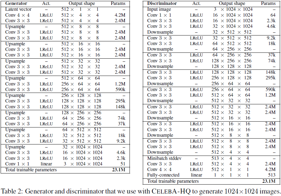
(2018,ProGAN)渐进式发展 GAN 以提高质量、稳定性和变化
Progressive Growing of GANs for Improved Quality, Stability, and Variation 公众号:EDPJ 目录 0. 摘要 1. 简介 2. GAN 的渐进式发展 3. 使用小批量标准差增加变化 4. 生成器和判别器的归一化 4.1 均衡学习率 4.2 生成器中的像素特征向量归一化 5. 评…...
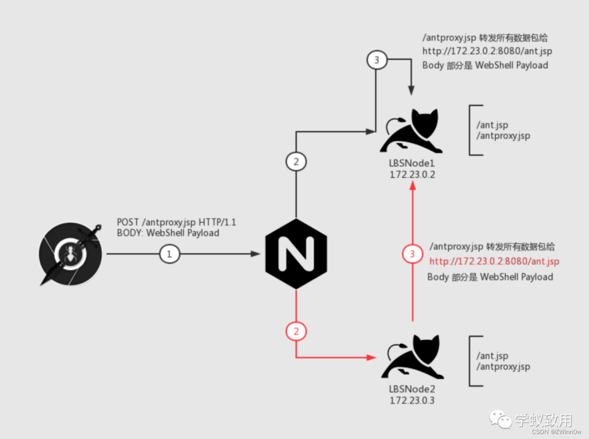
负载均衡下的 WebShell 连接
目录 负载均衡简介负载均衡的分类网络通信分类 负载均衡下的 WebShell 连接场景描述难点介绍解决方法**Plan A** **关掉其中一台机器**(作死)**Plan B** **执行前先判断要不要执行****Plan C** 在Web 层做一次 HTTP 流量转发 (重点࿰…...

Postman的高级用法—Runner的使用
1.首先在postman新建要批量运行的接口文件夹,新建一个接口,并设置好全局变量。 2.然后在Test里面设置好要断言的方法 如: tests["Status code is 200"] responseCode.code 200; tests["Response time is less than 10000…...

spring如何进行依赖注入,通过set方法把Dao注入到serves
1、选择Generate右键鼠标 你在service层后面方法的这些: 2、UserService配置文件的写法是怎样的: 3、我们在UserController中执行一下具体写法: 最后我们执行一下 : 4、这里可能出现空指针,因为你当前web层,因为你new这个对象根…...
和NumPy库来比较两副图像的相似度)
Python使用图像处理库PIL(Python Imaging Library)和NumPy库来比较两副图像的相似度
目录 1、解释说明: 2、使用示例: 3、注意事项: 1、解释说明: 在Python中,我们可以使用图像处理库PIL(Python Imaging Library)和NumPy库来比较两副图像的相似度。常用的图像相似度计算方法有…...

clickhouse扩缩容
一、背景 我们之前已经学会了搭建clickhouse集群,我们搭建的是一套单分片两副本的集群,接下来我们来测试下clickhouse的扩缩容情况 二、扩容 扩容相对来说比较简单,我们原来的架构如下 hostshardreplica192.169.1.111192.169.1.212 现在…...

动漫3D虚拟人物制作为企业数字化转型提供强大动力
一个 3D 虚拟数字人角色的制作流程,可以分为概念设定-3D 建模-贴图-蒙皮-动画-引擎测试六个步骤,涉及到的岗位有原画师、模型师、动画师等。角色概念设定、贴图绘制一般是由视觉设计师来完成;而建模、装配(骨骼绑定)、渲染动画是由三维设计师来制作完成。…...

数据同步工具比较:选择适合您业务需求的解决方案
在当今数字化时代,数据已经成为企业的核心资产。然而,随着业务的扩展和设备的增多,如何实现数据的高效管理和同步成为了一个亟待解决的问题。本文将介绍几种常见的数据同步工具,并对比它们的功能、性能和适用场景,帮助…...

Python中数据结构列表详解
列表是最常用的 Python 数据类型,它用一个方括号内的逗号分隔值出现,列表的数据项不需要具有相同的类型。 列表中的每个值都有对应的位置值,称之为索引,第一个索引是 0,第二个索引是 1,依此类推。列表都可…...

引领行业高质量发展|云畅科技参编《低代码开发平台创新发展路线图(2023)》
8月8日-9日,中国电子技术标准化研究院于北京顺利召开《低代码开发平台创新发展路线图(2023)》封闭编制会。云畅科技、浪潮、百度、广域铭岛等来自低代码开发平台解决方案供应商、用户方、科研院所等近30家相关单位的40余位专家参与了现场编制…...

Ubuntu22.04编译Nginx源码
执行如下命令 # ./configure --sbin-path/usr/local/nginx/nginx --conf-path/usr/local/nginx/nginx.conf --pid-path/usr/local/nginx/nginx.pid输出结果,出现如下: Configuration summary using system PCRE2 library OpenSSL library is not used …...

视频上传,限制时长,获取视频时长
使用element的upload上传文件时,除了类型和大小,需求需要限制只能长传18秒内的视频,这里通过upload的before-upload,以及创建一个音频元素对象拿到durtaion时长属性来实现。 getVideoTime(file) {return new Promise(async (resol…...

Open3D 进阶(5)变分贝叶斯高斯混合点云聚类
目录 一、算法原理二、代码实现三、结果展示四、测试数据本文由CSDN点云侠原创,原文链接。如果你不是在点云侠的博客中看到该文章,那么此处便是不要脸的爬虫。 系列文章(连载中。。。爬虫,你倒是爬个完整的呀?): Open3D 进阶(1) MeanShift点云聚类Open3D 进阶(2)DB…...

5、css学习5(链接、列表)
1、css可以设置链接的四种状态样式。 a:link - 正常,未访问过的链接a:visited - 用户已访问过的链接a:hover - 当用户鼠标放在链接上时a:active - 链接被点击的那一刻 2、 a:hover 必须在 a:link 和 a:visited 之后, a:active 必须在 a:hover 之后&…...
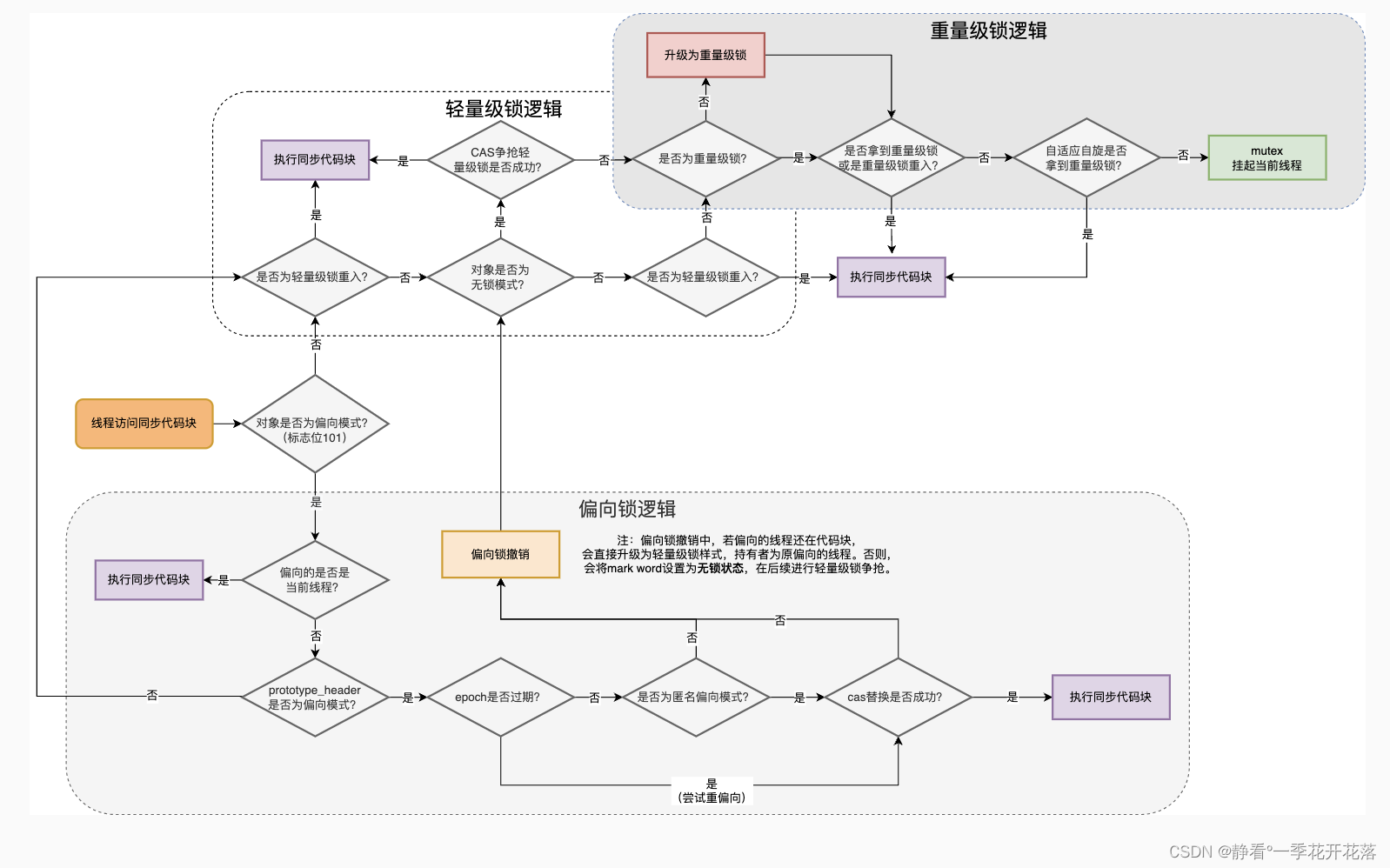
Synchronized与Java线程的关系
前言 Java多线程处理任务时,为了线程安全,通常会对共享资源进行加锁,拿到锁的线程才能进行访问共享资源。而加锁方式通过都是Synchronized锁或者Lock锁。 那么多线程在协同工作的时候,线程状态的变化都与锁对象有关系。 …...
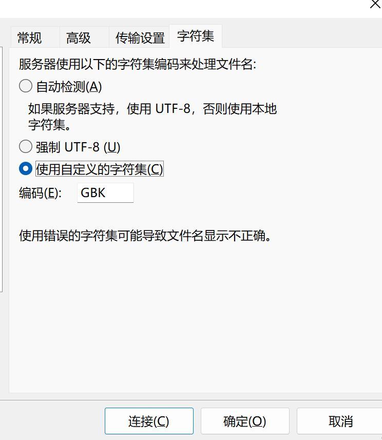
使用本地电脑搭建可以远程访问的SFTP服务器
文章目录 1. 搭建SFTP服务器1.1 下载 freesshd 服务器软件1.3 启动SFTP服务1.4 添加用户1.5 保存所有配置 2. 安装SFTP客户端FileZilla测试2.1 配置一个本地SFTP站点2.2 内网连接测试成功 3. 使用cpolar内网穿透3.1 创建SFTP隧道3.2 查看在线隧道列表 4. 使用SFTP客户端&#x…...
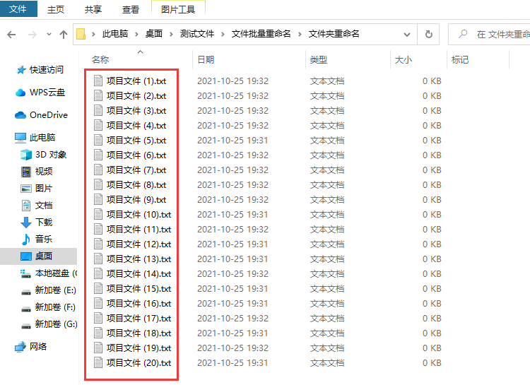
批量修改文件名怎么操作?
批量修改文件名怎么操作?不管你使用电脑处理工作还是进行学习,都会在电脑中产生很多的文件,时间一久电脑里的文件更加杂乱无章,这时候如果不对电脑中的文件进行及时的管理,那么很可能出现文件丢失而你自己还发现不了的…...

Chapter03-Authentication vulnerabilities
文章目录 1. 身份验证简介1.1 What is authentication1.2 difference between authentication and authorization1.3 身份验证机制失效的原因1.4 身份验证机制失效的影响 2. 基于登录功能的漏洞2.1 密码爆破2.2 用户名枚举2.3 有缺陷的暴力破解防护2.3.1 如果用户登录尝试失败次…...
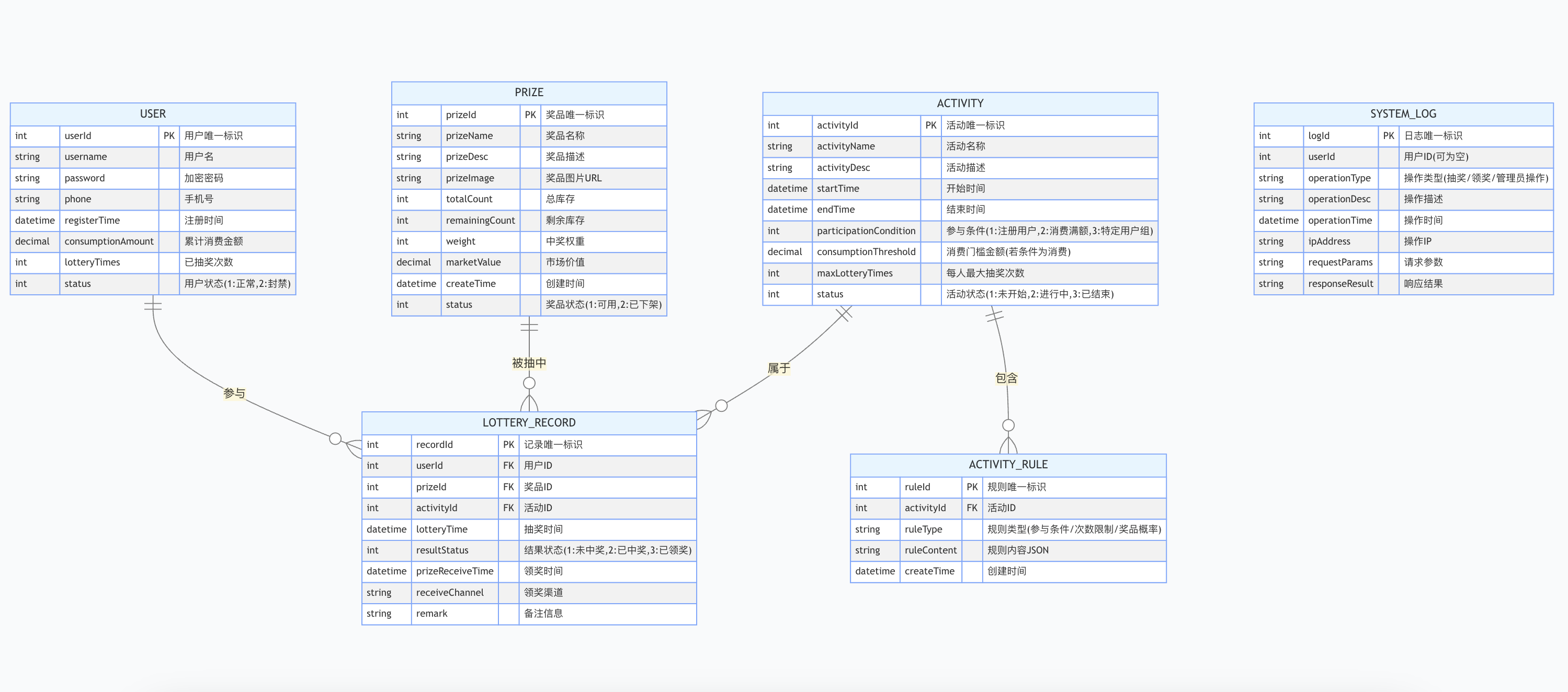
简易版抽奖活动的设计技术方案
1.前言 本技术方案旨在设计一套完整且可靠的抽奖活动逻辑,确保抽奖活动能够公平、公正、公开地进行,同时满足高并发访问、数据安全存储与高效处理等需求,为用户提供流畅的抽奖体验,助力业务顺利开展。本方案将涵盖抽奖活动的整体架构设计、核心流程逻辑、关键功能实现以及…...
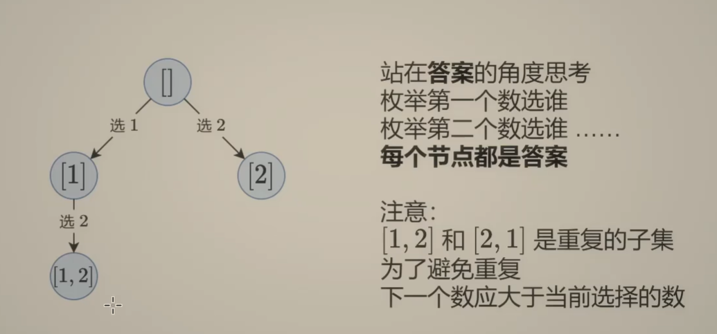
Day131 | 灵神 | 回溯算法 | 子集型 子集
Day131 | 灵神 | 回溯算法 | 子集型 子集 78.子集 78. 子集 - 力扣(LeetCode) 思路: 笔者写过很多次这道题了,不想写题解了,大家看灵神讲解吧 回溯算法套路①子集型回溯【基础算法精讲 14】_哔哩哔哩_bilibili 完…...

Linux简单的操作
ls ls 查看当前目录 ll 查看详细内容 ls -a 查看所有的内容 ls --help 查看方法文档 pwd pwd 查看当前路径 cd cd 转路径 cd .. 转上一级路径 cd 名 转换路径 …...
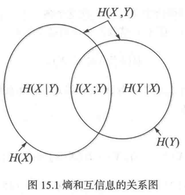
《通信之道——从微积分到 5G》读书总结
第1章 绪 论 1.1 这是一本什么样的书 通信技术,说到底就是数学。 那些最基础、最本质的部分。 1.2 什么是通信 通信 发送方 接收方 承载信息的信号 解调出其中承载的信息 信息在发送方那里被加工成信号(调制) 把信息从信号中抽取出来&am…...

Linux云原生安全:零信任架构与机密计算
Linux云原生安全:零信任架构与机密计算 构建坚不可摧的云原生防御体系 引言:云原生安全的范式革命 随着云原生技术的普及,安全边界正在从传统的网络边界向工作负载内部转移。Gartner预测,到2025年,零信任架构将成为超…...
使用 SymPy 进行向量和矩阵的高级操作
在科学计算和工程领域,向量和矩阵操作是解决问题的核心技能之一。Python 的 SymPy 库提供了强大的符号计算功能,能够高效地处理向量和矩阵的各种操作。本文将深入探讨如何使用 SymPy 进行向量和矩阵的创建、合并以及维度拓展等操作,并通过具体…...

MySQL账号权限管理指南:安全创建账户与精细授权技巧
在MySQL数据库管理中,合理创建用户账号并分配精确权限是保障数据安全的核心环节。直接使用root账号进行所有操作不仅危险且难以审计操作行为。今天我们来全面解析MySQL账号创建与权限分配的专业方法。 一、为何需要创建独立账号? 最小权限原则…...

安宝特方案丨船舶智造的“AR+AI+作业标准化管理解决方案”(装配)
船舶制造装配管理现状:装配工作依赖人工经验,装配工人凭借长期实践积累的操作技巧完成零部件组装。企业通常制定了装配作业指导书,但在实际执行中,工人对指导书的理解和遵循程度参差不齐。 船舶装配过程中的挑战与需求 挑战 (1…...

Java求职者面试指南:Spring、Spring Boot、MyBatis框架与计算机基础问题解析
Java求职者面试指南:Spring、Spring Boot、MyBatis框架与计算机基础问题解析 一、第一轮提问(基础概念问题) 1. 请解释Spring框架的核心容器是什么?它在Spring中起到什么作用? Spring框架的核心容器是IoC容器&#…...