《Python深度学习-Keras》精华笔记3:解决深度学习多分类问题
公众号:机器学习杂货店
作者:Peter
编辑:Peter
持续更新《Python深度学习》一书的精华内容,仅作为学习笔记分享。

本文是第三篇:介绍如何使用Keras解决Python深度学习中的多分类问题。
多分类问题和二分类问题的区别注意两点:
- 最后一层的激活函数使用softmax函数输出预测类别的概率,最大概率所在的位置就是预测的类别
- 损失函数使用分类交叉熵-categorical_crossentropy(针对0-1标签),整数标签使用(sparse_categorical_crossentropy)
运行环境:Python3.9.13 + Keras2.12.0 + tensorflow2.12.0
导入数据
机器学习中的路透社数据集是一个非常常用的数据集,它包含来自新闻专线的文本数据,主要用于文本分类任务。这个数据集是由路透社新闻机构提供的,包含了大量的新闻文章,共计22类分类标签。
- 该数据集的每一条新闻文章都被标记了一个或多个分类标签,这些标签表明了新闻文章的主题或类别。例如,政治、经济、体育、科技等。数据集中的每条新闻都包含文本内容和对应的分类标签,这使得路透社数据集成为机器学习领域中一个非常有价值的数据集。
- 路透社数据集的挑战在于数据的复杂性、多样性和快速变化。新闻文章具有各种不同的语言和格式,包括标题、段落、列表和图片等。此外,新闻文章的表述方式也各不相同,包括情感、风格和话题等。因此,路透社数据集的难度较高,需要机器学习算法具备高水平的分类能力。
- 路透社数据集在机器学习领域中得到了广泛应用,主要用于评估和提升文本分类算法的性能。许多机器学习算法,包括支持向量机、决策树、随机森林和神经网络等,都曾在路透社数据集上进行过测试和比较。因此,该数据集被广泛用于评估文本分类算法的性能,并已成为机器学习领域中的经典数据集之一。
In [1]:
import numpy as np
np.random.seed(1234)import warnings
warnings.filterwarnings("ignore")
训练集和标签
In [2]:
from keras.datasets import reuters
In [3]:
# 取出数据中前10000个词语(train_data, train_labels), (test_data, test_labels) = reuters.load_data(num_words=10000)
数据查看
In [4]:
train_data[:2]
Out[4]:
array([list([1, 2, 2, 8, 43, 10, 447, 5, 25, 207, 270, 5, 3095, 111, 16, 369, 186, 90, 67, 7, 89, 5, 19, 102, 6, 19, 124, 15, 90, 67, 84, 22, 482, 26, 7, 48, 4, 49, 8, 864, 39, 209, 154, 6, 151, 6, 83, 11, 15, 22, 155, 11, 15, 7, 48, 9, 4579, 1005, 504, 6, 258, 6, 272, 11, 15, 22, 134, 44, 11, 15, 16, 8, 197, 1245, 90, 67, 52, 29, 209, 30, 32, 132, 6, 109, 15, 17, 12]),list([1, 3267, 699, 3434, 2295, 56, 2, 7511, 9, 56, 3906, 1073, 81, 5, 1198, 57, 366, 737, 132, 20, 4093, 7, 2, 49, 2295, 2, 1037, 3267, 699, 3434, 8, 7, 10, 241, 16, 855, 129, 231, 783, 5, 4, 587, 2295, 2, 2, 775, 7, 48, 34, 191, 44, 35, 1795, 505, 17, 12])],dtype=object)
In [5]:
len(train_data), len(test_data)
Out[5]:
(8982, 2246)
查看label中数据信息:总共是46个类别
In [6]:
train_labels[:20]
Out[6]:
array([ 3, 4, 3, 4, 4, 4, 4, 3, 3, 16, 3, 3, 4, 4, 19, 8, 16,3, 3, 21], dtype=int64)
In [7]:
test_labels[:20]
Out[7]:
array([ 3, 10, 1, 4, 4, 3, 3, 3, 3, 3, 5, 4, 1, 3, 1, 11, 23,3, 19, 3], dtype=int64)
单词和索引的互换:
In [8]:
word_index = reuters.get_word_index()reverse_word_index = dict([value, key] for (key, value) in word_index.items())  # 翻转过程
decoded_review = ' '.join([reverse_word_index.get(i-3, "?") for i in train_data[0]])
decoded_review
Out[8]:
'? ? ? said as a result of its december acquisition of space co it expects earnings per share in 1987 of 1 15 to 1 30 dlrs per share up from 70 cts in 1986 the company said pretax net should rise to nine to 10 mln dlrs from six mln dlrs in 1986 and rental operation revenues to 19 to 22 mln dlrs from 12 5 mln dlrs it said cash flow per share this year should be 2 50 to three dlrs reuter 3'
数据向量化
关于数据向量化的过程:
In [9]:
# 同样的向量化函数import numpy as npdef vectorszie(seq, dim=10000): """seq: 输入序列dim:10000,维度"""results = np.zeros((len(seq), dim)) # 创建全0矩阵 length * dimfor i, s in enumerate(seq):results[i,s] = 1. # 将该位置的值从0变成1,如果没有出现则还是0return results
In [10]:
# 两个数据向量化x_train = vectorszie(train_data)
x_test = vectorszie(test_data)
标签向量化
针对标签向量化方法1:自定义独热编码函数
In [11]:
# 1、手动实现def to_one_hot(labels, dimension=10000):results = np.zeros((len(labels), dimension))  # 全0矩阵 np.zeros((m, n))for i, label in enumerate(labels):results[i,labels] = 1.  # 一定是浮点数return results # 调用定义的函数
one_hot_train_labels = to_one_hot(train_labels)
one_hot_test_labels = to_one_hot(test_labels)
针对标签向量化方法2:基于keras内置函数来实现
In [12]:
# keras内置方法
from keras.utils.np_utils import to_categoricalone_hot_train_labels = to_categorical(train_labels)
one_hot_test_labels = to_categorical(test_labels)
整数标签处理(基于sparse_categorical_crossentropy)
如果我们不想将分类标签(46个取值)转成独热码形式,可以使用稀疏分类标签:sparse_categorical_crossentropy。
使用方法都是类似的:
y_train = np.array(train_labels)
y_test = np.array(test_labels)model.compile(optimizer='rmsprop',  # 优化器loss='sparse_categorical_crossentropy',  # 稀疏分类损失metrics=['accuracy']   # 评价指标)
训练集和验证集
In [13]:
#  取出1000个样本作为验证集x_val = x_train[:1000]
part_x_train = x_train[1000:]y_val = one_hot_train_labels[:1000]
part_y_train = one_hot_train_labels[1000:]
构建网络
In [14]:
from keras import models
from keras import layersmodel = models.Sequential()
model.add(layers.Dense(64, activation='relu', input_shape=(x_train.shape[1],)))  #  X_train.shape[1] = 10000
model.add(layers.Dense(64,activation="relu"))
model.add(layers.Dense(46, activation="softmax"))    #  46就是最终的分类数目
对比二分类问题,有3个需要注意的点:
- 网络的第一层输入的𝑠ℎ𝑎𝑝𝑒shape为𝑥𝑡𝑟𝑎𝑖𝑛xtrain的𝑠ℎ𝑎𝑝𝑒shape第二个值
- 网络的最后一个层是4646的𝐷𝑒𝑛𝑠𝑒Dense层(标签有46个类别);网络输出的是一个46维的向量。向量中每个元素代表不同的类别的输出概率。
- 采用的激活函数是𝑠𝑜𝑓𝑡𝑚𝑎𝑥softmax函数(二分类是𝑠𝑖𝑔𝑚𝑜𝑖𝑑sigmoid函数);在输出向量中的元素代表每个类别的概率,概率之和为1;𝑜𝑢𝑡𝑝𝑢𝑡[𝑖]output[i]表示第𝑖i类的概率。
编译网络
In [15]:
model.compile(optimizer='rmsprop', # 优化器loss='categorical_crossentropy', # 多分类交叉熵categorical_crossentropymetrics=['accuracy'] # 评价指标)
In [16]:
## 训练网络
In [17]:
history = model.fit(part_x_train,  # inputpart_y_train,  # outputepochs=20,  # 训练20个轮次batch_size=512,  # 每次迭代使用512个样本的小批量validation_data=[x_val,y_val]   # 验证集的数据)
Epoch 1/20
16/16 [==============================] - 1s 26ms/step - loss: 2.6860 - accuracy: 0.4868 - val_loss: 1.8084 - val_accuracy: 0.6240
Epoch 2/20
16/16 [==============================] - 0s 14ms/step - loss: 1.5509 - accuracy: 0.6750 - val_loss: 1.3812 - val_accuracy: 0.6850
Epoch 3/20
16/16 [==============================] - 0s 14ms/step - loss: 1.2006 - accuracy: 0.7357 - val_loss: 1.1962 - val_accuracy: 0.7300
......
Epoch 18/20
16/16 [==============================] - 0s 14ms/step - loss: 0.1567 - accuracy: 0.9559 - val_loss: 0.9402 - val_accuracy: 0.8110
Epoch 19/20
16/16 [==============================] - 0s 14ms/step - loss: 0.1439 - accuracy: 0.9559 - val_loss: 0.9561 - val_accuracy: 0.8040
Epoch 20/20
16/16 [==============================] - 0s 13ms/step - loss: 0.1401 - accuracy: 0.9546 - val_loss: 0.9467 - val_accuracy: 0.8090
模型概览
In [18]:
model.summary()
Model: "sequential"
_________________________________________________________________Layer (type)                Output Shape              Param #
=================================================================dense (Dense)               (None, 64)                640064    dense_1 (Dense)             (None, 64)                4160      dense_2 (Dense)             (None, 46)                2990      =================================================================
Total params: 647,214
Trainable params: 647,214
Non-trainable params: 0
_________________________________________________________________
模型指标评估
In [19]:
x_test
Out[19]:
array([[0., 1., 1., ..., 0., 0., 0.],[0., 1., 1., ..., 0., 0., 0.],[0., 1., 1., ..., 0., 0., 0.],...,[0., 1., 0., ..., 0., 0., 0.],[0., 1., 1., ..., 0., 0., 0.],[0., 1., 1., ..., 0., 0., 0.]])
In [20]:
one_hot_test_labels
Out[20]:
array([[0., 0., 0., ..., 0., 0., 0.],[0., 0., 0., ..., 0., 0., 0.],[0., 1., 0., ..., 0., 0., 0.],...,[0., 0., 0., ..., 0., 0., 0.],[0., 0., 0., ..., 0., 0., 0.],[0., 0., 0., ..., 0., 0., 0.]], dtype=float32)
In [21]:
# one_hot_test_labels 经历了独热编码后的labelsmodel.evaluate(x_test, one_hot_test_labels)
71/71 [==============================] - 0s 1ms/step - loss: 1.0572 - accuracy: 0.7872
Out[21]:
[1.0572034120559692, 0.7871772050857544]
模型指标可视化
In [22]:
his_dict = history.history  # 字典类型
his_dict.keys()
Out[22]:
dict_keys(['loss', 'accuracy', 'val_loss', 'val_accuracy'])
In [23]:
import matplotlib.pyplot as pltloss = his_dict["loss"]
val_loss = his_dict["val_loss"]
acc = his_dict["accuracy"]
val_acc = his_dict["val_accuracy"]
In [24]:
epochs = range(1, len(loss) + 1)  # 作为横轴# 1、损失lossplt.plot(epochs, loss, "bo", label="Training Loss")
plt.plot(epochs, val_loss, "b", label="Validation Loss")
plt.xlabel("Epochs")
plt.ylabel("Loss")
plt.legend()
plt.title("Training and Validation Loss")
plt.show()
针对精度的可视化过程:
In [25]:
# 2、精度accplt.clf()  #  清空图像
plt.plot(epochs, acc, "bo", label="Training Acc")
plt.plot(epochs, val_acc, "b", label="Validation Acc")
plt.xlabel("Epochs")
plt.ylabel("Acc")
plt.legend()plt.title("Training and Validation Acc")
plt.show()
重新训练
可以看到loss在训练集上逐渐减小的;但是在验证集上到达第8轮后保持不变;精度acc也在训练集上表现良好,但是在验证集上在第9轮后基本不变。
显然是出现了过拟合。我们重新训练指定9轮
指定轮次训练
In [26]:
from keras.datasets import reuters
import numpy as np# 取出数据中前10000个词语
(train_data, train_labels), (test_data, test_labels) = reuters.load_data(num_words=10000)def vectorszie(seq, dim=10000):  """seq: 输入序列dim:10000,维度"""results = np.zeros((len(seq), dim))  # 创建全0矩阵  length * dimfor i, s in enumerate(seq):results[i,s] = 1.   # 将该位置的值从0变成1,如果没有出现则还是0return results# 两个数据向量化
x_train = vectorszie(train_data)
x_test = vectorszie(test_data)  # one-hot编码
from keras.utils.np_utils import to_categorical
one_hot_train_labels = to_categorical(train_labels)
one_hot_test_labels = to_categorical(test_labels)#  取出1000个样本作为验证集
x_val = x_train[:1000]
part_x_train = x_train[1000:]
y_val = one_hot_train_labels[:1000]
part_y_train = one_hot_train_labels[1000:]# 构建网络
from keras import models
from keras import layersmodel = models.Sequential()
model.add(layers.Dense(64, activation='relu', input_shape=(x_train.shape[1],)))  #  X_train.shape[1] = 10000
model.add(layers.Dense(64,activation="relu"))
model.add(layers.Dense(46, activation="softmax"))    #  46就是最终的分类数目# 模型编译
model.compile(optimizer='rmsprop',  # 优化器loss='categorical_crossentropy',  # 多分类交叉熵categorical_crossentropymetrics=['accuracy']   # 评价指标)model.fit(part_x_train,  # inputpart_y_train,  # outputepochs=9,  # 训练个9轮次verbose=0,  # 是否显示训练细节batch_size=512,  # 每次迭代使用512个样本的小批量validation_data=[x_val,y_val]   # 验证集的数据)# 模型评估
model.evaluate(x_test, one_hot_test_labels)
71/71 [==============================] - 0s 1ms/step - loss: 0.9535 - accuracy: 0.7801
Out[26]:
[0.9534968733787537, 0.780053436756134]
可以看到精度接近79%
确定预测类别
如何查看预测类别?以第一个数据的预测结果为例:
In [27]:
results = model.predict(x_test)
results
71/71 [==============================] - 0s 997us/step
Out[27]:
array([[5.1504822e-04, 1.0902017e-04, 2.1993063e-04, ..., 1.9025596e-05,4.6712950e-07, 3.7851787e-05],[5.1406571e-03, 4.2032253e-02, 1.9307269e-03, ..., 1.3830569e-02,5.6258432e-04, 3.1604938e-04],[4.0979325e-03, 7.7002281e-01, 6.7354720e-03, ..., 1.8014901e-03,4.9561085e-03, 9.9538732e-04],...,[6.1581237e-04, 1.1025119e-03, 3.9810984e-04, ..., 2.9050951e-05,2.4186371e-05, 6.5296721e-05],[3.6575866e-03, 1.0463378e-02, 3.1981221e-03, ..., 2.7204564e-04,9.7423712e-05, 1.8902053e-03],[1.8005458e-03, 7.0240724e-01, 1.8455695e-02, ..., 1.9976693e-04,5.6885678e-04, 1.8073655e-04]], dtype=float32)
In [28]:
predict_one = results[0]
predict_one
Out[28]:
array([5.1504822e-04, 1.0902017e-04, 2.1993063e-04, 3.9642093e-01,5.7400799e-01, 1.5043363e-04, 4.0421914e-05, 7.1661170e-06,3.2984249e-03, 1.5247319e-04, 3.9692928e-05, 3.0673095e-03,1.3204347e-03, 3.9371965e-04, 2.1458001e-04, 1.5276371e-04,1.8565950e-03, 1.2035699e-04, 6.1764423e-04, 7.4270181e-03,3.6794273e-03, 2.7725848e-03, 2.1595537e-05, 7.5044850e-04,1.5939959e-05, 3.3097478e-04, 9.2904102e-06, 1.1782978e-04,3.3141983e-05, 2.0210361e-04, 4.8371754e-04, 2.3283543e-04,5.7479672e-05, 3.8166454e-05, 9.9279227e-05, 3.2270618e-05,2.8716330e-04, 3.2858396e-05, 1.2131617e-05, 3.3482770e-04,9.0265028e-05, 1.7225980e-04, 4.2123888e-06, 1.9025596e-05,4.6712950e-07, 3.7851787e-05], dtype=float32)
In [29]:
len(predict_one) # 总长度是46
Out[29]:
46
In [30]:
np.sum(predict_one) # 预测总和是1
Out[30]:
1.0000002
如何找到哪个概率最大的元素所在的位置索引?使用np.argmax函数。该位置索引就是预测的最终类别。
In [31]:
np.argmax(predict_one)
Out[31]:
4
所以第一个数据预测的类别是第3类。
所有测试集的预测结果:
In [32]:
# 基于列表推导式# 预测值
y_predict = [np.argmax(result) for result in results]
y_predict[:20]
Out[32]:
[4, 10, 1, 4, 13, 3, 3, 3, 3, 3, 1, 4, 1, 3, 1, 11, 4, 3, 19, 3]
In [33]:
test_labels[:20] # 真实值
Out[33]:
array([ 3, 10, 1, 4, 4, 3, 3, 3, 3, 3, 5, 4, 1, 3, 1, 11, 23,3, 19, 3], dtype=int64)
In [34]:
from sklearn.metrics import classification_report, confusion_matrix, r2_score, recall_score, accuracy_score
In [35]:
# 精度、R2print("多分类预测建模的精度acc为: ",accuracy_score(test_labels,y_predict))
print("多分类预测建模的R方为: ",r2_score(test_labels, y_predict))
# print("多分类预测的报告: \n",classification_report(y_predict, test_labels))
多分类预测建模的精度acc为:  0.780053428317008
多分类预测建模的R方为:  0.4157152870789089
预测的精度为78%左右
预测结果统计
根据预测结果和真实值,从头实现精度的计算,不调用任何相关模块。
In [36]:
import pandas as pddf = pd.DataFrame({"y_test":test_labels,"y_predict":y_predict})df.head()
Out[36]:
| y_test | y_predict | |
|---|---|---|
| 0 | 3 | 4 |
| 1 | 10 | 10 |
| 2 | 1 | 1 |
| 3 | 4 | 4 |
| 4 | 4 | 13 |
In [37]:
df["result"] = (df["y_test"] == df["y_predict"])  # 判断相等为True  否则为False
df.head()
Out[37]:
| y_test | y_predict | result | |
|---|---|---|---|
| 0 | 3 | 4 | False |
| 1 | 10 | 10 | True |
| 2 | 1 | 1 | True |
| 3 | 4 | 4 | True |
| 4 | 4 | 13 | False |
统计不同原标签的正确预测数目:sum求和只对True(变成1),False为0
In [38]:
df1 = df.groupby("y_test")["result"].sum()
df1.head(10)
Out[38]:
y_test
0      7
1     84
2     12
3    744
4    437
5      0
6     12
7      1
8     23
9     16
Name: result, dtype: int64
In [39]:
df1.sort_values(ascending=False).head(10)
Out[39]:
y_test
3     744
4     437
19     96
1      84
16     75
11     68
20     34
10     25
8      23
13     22
Name: result, dtype: int64
可以看到第3、4、19类别是预测准确最多的。原始数据中每个类别的数目:
In [40]:
df2 = df["y_test"].value_counts().sort_index()
df2.head(10)
Out[40]:
0     12
1    105
2     20
3    813
4    474
5      5
6     14
7      3
8     38
9     25
Name: y_test, dtype: int64
In [41]:
df1.values
Out[41]:
array([ 7, 84, 12, 744, 437, 0, 12, 1, 23, 16, 25, 68, 0,22, 0, 1, 75, 2, 12, 96, 34, 18, 0, 3, 4, 20,4, 1, 1, 0, 6, 2, 6, 1, 5, 0, 2, 0, 0,0, 0, 1, 0, 3, 4, 0], dtype=int64)
In [42]:
# 将df1-df2合并df3 = pd.DataFrame({"predict":df1.values,  # 预测正确数目"true":df2.values})  # 原数据数目
df3.head()
Out[42]:
| predict | true | |
|---|---|---|
| 0 | 7 | 12 |
| 1 | 84 | 105 |
| 2 | 12 | 20 |
| 3 | 744 | 813 |
| 4 | 437 | 474 |
In [43]:
df3["precision"] = df3["predict"] / df3["true"]
df3.head(10)
Out[43]:
| predict | true | precision | |
|---|---|---|---|
| 0 | 7 | 12 | 0.583333 |
| 1 | 84 | 105 | 0.800000 |
| 2 | 12 | 20 | 0.600000 |
| 3 | 744 | 813 | 0.915129 |
| 4 | 437 | 474 | 0.921941 |
| 5 | 0 | 5 | 0.000000 |
| 6 | 12 | 14 | 0.857143 |
| 7 | 1 | 3 | 0.333333 |
| 8 | 23 | 38 | 0.605263 |
| 9 | 16 | 25 | 0.640000 |
可以和分类报告中的precision进行对比,结果是一致的(除去小数位问题)
In [44]:
print("多分类预测的报告: \n",classification_report(y_predict, test_labels))# 结果(部分)
多分类预测的报告: precision    recall  f1-score   support0       0.58      0.88      0.70         81       0.80      0.60      0.68       1412       0.60      0.86      0.71        143       0.92      0.94      0.93       7884       0.92      0.75      0.82       5865       0.00      0.00      0.00         06       0.86      0.80      0.83        157       0.33      1.00      0.50         18       0.61      0.70      0.65        339       0.64      0.84      0.73        1910       0.83      0.81      0.82        3111       0.82      0.51      0.63       13312       0.00      0.00      0.00         213       0.59      0.61      0.60        3614       0.00      0.00      0.00         015       0.11      0.50      0.18         216       0.76      0.72      0.74       10417       0.17      1.00      0.29         218       0.60      0.60      0.60        20
相关文章:
《Python深度学习-Keras》精华笔记3:解决深度学习多分类问题
公众号:机器学习杂货店作者:Peter编辑:Peter 持续更新《Python深度学习》一书的精华内容,仅作为学习笔记分享。 本文是第三篇:介绍如何使用Keras解决Python深度学习中的多分类问题。 多分类问题和二分类问题的区别注意…...

区块链世界的大数据入门之zkMapReduce简介
1. 引言 跨链互操作性的未来将围绕多链dapp之间的动态和数据丰富的关系构建。Lagrange Labs 正在构建粘合剂,以帮助安全地扩展基于零知识证明的互操作性。 2. ZK大数据栈 Lagrange Labs 的ZK大数据栈 为一种专有的证明结构,用于在任意动态分布式计算的…...

Python流程控制语句-条件判断语句练习及应用详解
文章目录 简介条件判断语句(if语句)练习1:判断奇偶数练习2:判断闰年练习3:计算狗的年龄相当于人的年龄练习4:根据成绩奖励练习5:选择婚姻对象 小结 python 学习专栏推荐python基础知识ÿ…...
ElasticSearch高级使用【别名,重建索引,refresh操作,高亮查询,查询建议】)
(十)ElasticSearch高级使用【别名,重建索引,refresh操作,高亮查询,查询建议】
1.别名使用 1)别名作用 在开发中,随着业务需求的迭代,较⽼的业务逻辑就要⾯临更新甚⾄是重构,⽽对于es来说,为了 适应新的业务逻辑,可能就要对原有的索引做⼀些修改,⽐如对某些字段做调整&…...

基于小波神经网络的中药材价格预测,基于ANN的小波神经网络中药材价格预测
目标 背影 BP神经网络的原理 BP神经网络的定义 BP神经网络的基本结构 BP神经网络的神经元 BP神经网络的激活函数, BP神经网络的传递函数 小波神经网络(以小波基为传递函数的BP神经网络) 代码链接:基于小波神经网络的中药材价格预测,ANN小波神经网络中药材价格预测资源-CS…...

thinkPhp5返回某些指定字段
//去除掉密码$db new UserModel();$result $db->field(password,true)->where("username{$params[username]} AND password{$params[password]}")->find(); 或者指定要的字段的数组 $db new UserModel();$result $db->field([username,create_time…...
基于docker环境的tomcat开启远程调试
背景: Tomcat部署在docker环境中,使用rancher来进行管理,需要对其进行远程调试。 操作步骤: 1.将容器中的catalina.sh映射出来,便于对其修改,添加远程调试相关参数。 注意:/data/produce2201…...
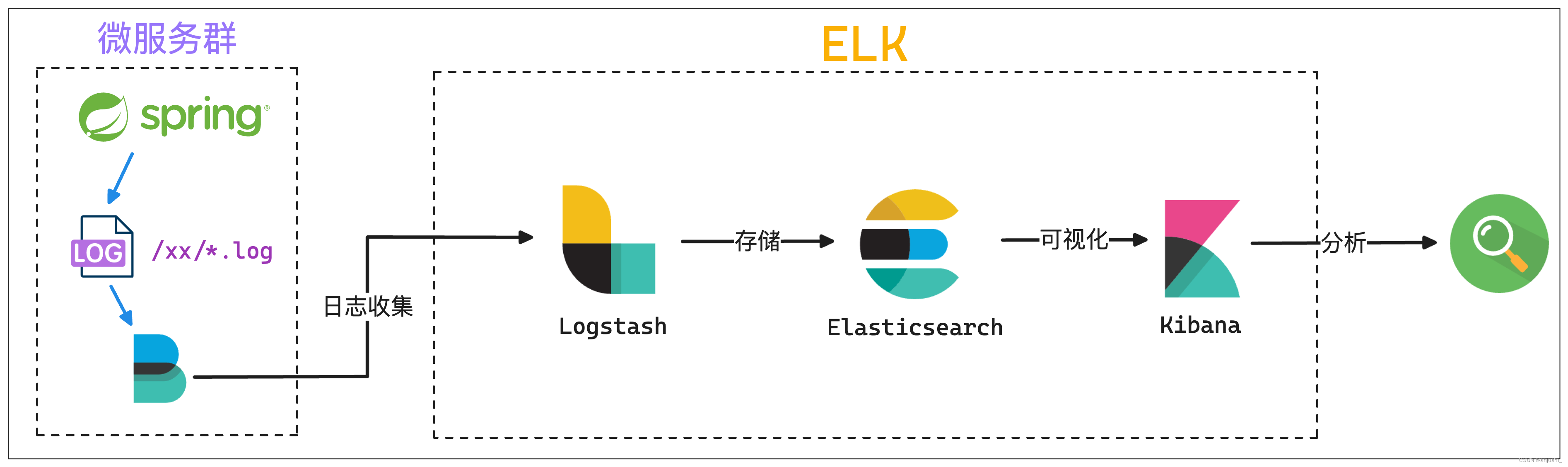
ELK日志框架图总结
ELK日志框架图总结 本文目录 ELK日志框架图总结Elastic Stack介绍模式分层图beatselasticsearchkibana模式logstashelasticsearchkibana模式beatslogstashelasticsearchkibana模式beats缓存/消息队列logstashelasticsearchkibana模式elkspringboot Elastic Stack介绍 官网&…...

go 每天定时任务 --chatGPT
问:clearLog(hour,cmds),定时执行shell 命令,hour 为每天的几点,cmds 为linux命令数组字符串(如 1,{"ls","cd"}) gpt: 要编写一个 Go 函数 clearLog,该函数可…...

Lightdb 23.3 plorasql函数支持DML
开篇立意 oracle在函数中使用dml语句时,有两者情况。即:(1)直接使用select调用该函数;(2)在匿名块中调用该函数。 针对第一种情况我们测试一下 简单的函数: create table nested_t…...

电容笔值不值得买?开学季比较好用的电容笔
眼看着新学期即将到来,到底应该选择什么样的电容笔?一款原装的苹果Pencil,就卖到了将近一千块,这对于很多人来说,都是一个十分昂贵的价格。事实上,由于平替电容笔的价格非常便宜,只要一二百元就…...
 分页)
Mybatis 框架 ( 五 ) 分页
4.6.分页 Mybatis-plus 内置分页插件, 并支持多种数据库 官网 : 分页插件 | MyBatis-Plus (baomidou.com) 4.6.1.增加拦截器 通过 MapperScan 指定 mapper接口的路径 import com.baomidou.mybatisplus.annotation.DbType; import com.baomidou.mybatisplus.extension.plug…...

Python模板注入
概念 发生在使用模板引擎解析用户提供的输入时。模板注入漏洞可能导致攻击者能够执行恶意代码或访问未授权的数据。 模板引擎可以让(网站)程序实现界面与数据分离,业务代码与逻辑代码分离。即也拓宽了攻击面,注入到模板中的代码可…...

Java常用的设计模式
单例模式(Singleton Pattern): 确保一个类只有一个实例,并提供一个全局访问点。示例:应用程序中的配置管理器。 工厂模式(Factory Pattern): 用于创建对象的模式,封装对象的创建过程。示例&…...
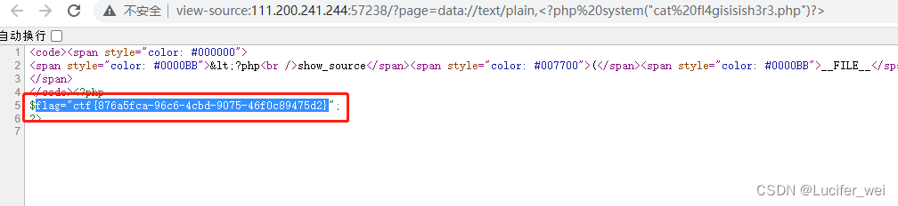
攻防世界-WEB-Web_php_include
打开靶机 通过代码审计可以知道,存在文件包含漏洞,并且对伪协议php://进行了过滤。 发现根目录下存在phpinfo 观察phpinfo发现如下: 这两个都为on 所以我们就可以使用data://伪协议 payload如下: - ?pagedata://text/plain,…...

angular中多层嵌套结构的表单如何处理回显问题
最近在处理angular表单时,有一个4层结构的表单。而且很多元素时动态生成,如下: this.validateFormthis.fb.group({storeId: ["test12"],storeNameKey:[],config:this.fb.group({ tableSize:this.fb.group({toggle:[false],groupSiz…...
Leetcode646. 最长数对链
Every day a Leetcode 题目来源:646. 最长数对链 解法1:动态规划 定义 dp[i] 为以 pairs[i] 为结尾的最长数对链的长度。 初始化时,dp 数组需要全部赋值为 1。 计算 dp[i] 时,可以先找出所有的满足 pairs[i][0]>pairs[j]…...

Windows 下安装NPM
第一步: 下载node.js的windows版 当前最新版本是https://nodejs.org/dist/ 第二步:设置环境变量 把node.exe所在目录加入到PATH环境变量中。 配置成功后可以在CMD中通过node --version 看到node.js对应的版本号 C:\Users\fn>node --version v6.10.2 第三步: 安装git 直接…...

【ARM CoreLink 系列 2 -- CCI-400 控制器简介】
文章目录 CCI-400 介绍DVM 机制介绍DVM 消息传输过程TOKEN 机制介绍 下篇文章:ARM CoreLink 系列 3 – CCI-550 控制器介绍 CCI-400 介绍 CCI(Cache Coherent Interconnect)是ARM 中 的Cache一致性控制器。 CCI-400 将 Interconnect 和coh…...
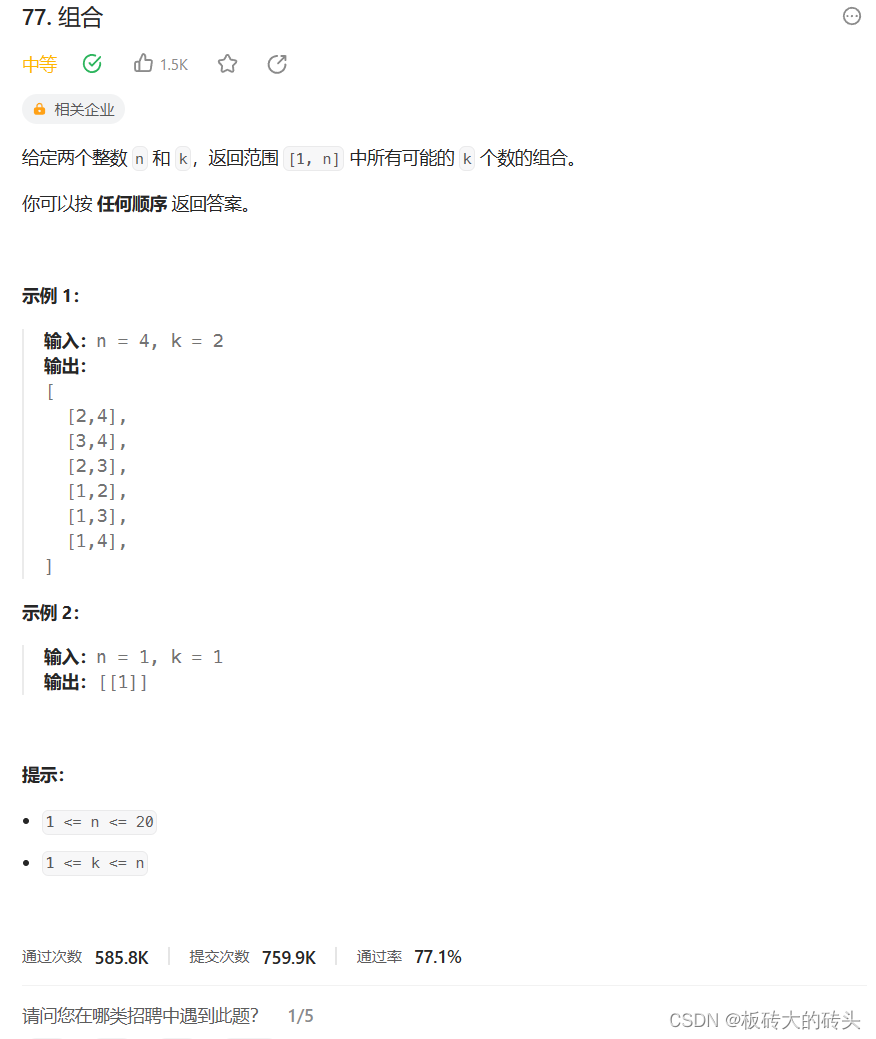
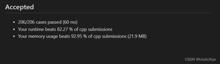
LeetCode(力扣)77. 组合Python
LeetCode77. 组合 题目链接代码 题目链接 https://leetcode.cn/problems/combinations/description/ 代码 class Solution:def combine(self, n: int, k: int) -> List[List[int]]:result []return self.backtracking(n, k, 1, [], result)def backtracking(self, n, k…...
` 方法)
深入浅出:JavaScript 中的 `window.crypto.getRandomValues()` 方法
深入浅出:JavaScript 中的 window.crypto.getRandomValues() 方法 在现代 Web 开发中,随机数的生成看似简单,却隐藏着许多玄机。无论是生成密码、加密密钥,还是创建安全令牌,随机数的质量直接关系到系统的安全性。Jav…...

智能在线客服平台:数字化时代企业连接用户的 AI 中枢
随着互联网技术的飞速发展,消费者期望能够随时随地与企业进行交流。在线客服平台作为连接企业与客户的重要桥梁,不仅优化了客户体验,还提升了企业的服务效率和市场竞争力。本文将探讨在线客服平台的重要性、技术进展、实际应用,并…...

五年级数学知识边界总结思考-下册
目录 一、背景二、过程1.观察物体小学五年级下册“观察物体”知识点详解:由来、作用与意义**一、知识点核心内容****二、知识点的由来:从生活实践到数学抽象****三、知识的作用:解决实际问题的工具****四、学习的意义:培养核心素养…...
cf2117E
原题链接:https://codeforces.com/contest/2117/problem/E 题目背景: 给定两个数组a,b,可以执行多次以下操作:选择 i (1 < i < n - 1),并设置 或,也可以在执行上述操作前执行一次删除任意 和 。求…...

【git】把本地更改提交远程新分支feature_g
创建并切换新分支 git checkout -b feature_g 添加并提交更改 git add . git commit -m “实现图片上传功能” 推送到远程 git push -u origin feature_g...
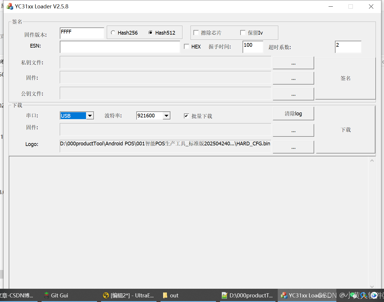
C++ Visual Studio 2017厂商给的源码没有.sln文件 易兆微芯片下载工具加开机动画下载。
1.先用Visual Studio 2017打开Yichip YC31xx loader.vcxproj,再用Visual Studio 2022打开。再保侟就有.sln文件了。 易兆微芯片下载工具加开机动画下载 ExtraDownloadFile1Info.\logo.bin|0|0|10D2000|0 MFC应用兼容CMD 在BOOL CYichipYC31xxloaderDlg::OnIni…...
相比,优缺点是什么?适用于哪些场景?)
Redis的发布订阅模式与专业的 MQ(如 Kafka, RabbitMQ)相比,优缺点是什么?适用于哪些场景?
Redis 的发布订阅(Pub/Sub)模式与专业的 MQ(Message Queue)如 Kafka、RabbitMQ 进行比较,核心的权衡点在于:简单与速度 vs. 可靠与功能。 下面我们详细展开对比。 Redis Pub/Sub 的核心特点 它是一个发后…...
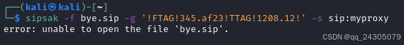
sipsak:SIP瑞士军刀!全参数详细教程!Kali Linux教程!
简介 sipsak 是一个面向会话初始协议 (SIP) 应用程序开发人员和管理员的小型命令行工具。它可以用于对 SIP 应用程序和设备进行一些简单的测试。 sipsak 是一款 SIP 压力和诊断实用程序。它通过 sip-uri 向服务器发送 SIP 请求,并检查收到的响应。它以以下模式之一…...

Redis:现代应用开发的高效内存数据存储利器
一、Redis的起源与发展 Redis最初由意大利程序员Salvatore Sanfilippo在2009年开发,其初衷是为了满足他自己的一个项目需求,即需要一个高性能的键值存储系统来解决传统数据库在高并发场景下的性能瓶颈。随着项目的开源,Redis凭借其简单易用、…...
c++第七天 继承与派生2
这一篇文章主要内容是 派生类构造函数与析构函数 在派生类中重写基类成员 以及多继承 第一部分:派生类构造函数与析构函数 当创建一个派生类对象时,基类成员是如何初始化的? 1.当派生类对象创建的时候,基类成员的初始化顺序 …...