斯坦福数据挖掘教程·第三版》读书笔记(英文版)Chapter 10 Mining Social-Network Graphs
来源:《斯坦福数据挖掘教程·第三版》对应的公开英文书和PPT。
Chapter 10 Mining Social-Network Graphs
The essential characteristics of a social network are:
- There is a collection of entities that participate in the network. Typically, these entities are people, but they could be something else entirely.
- There is at least one relationship between entities of the network. On Facebook or its ilk, this relationship is called friends. Sometimes the relationship is all-or-nothing; two people are either friends or they are not. However, in other examples of social networks, the relationship has a degree. This degree could be discrete; e.g., friends, family, acquaintances,
or none as in Google+. It could be a real number; an example would be the fraction of the average day that two people spend talking to each other. - There is an assumption of nonrandomness or locality. This condition is the hardest to formalize, but the intuition is that relationships tend to cluster. That is, if entity A is related to both B and C, then there is a higher probability than average that B and C are related.
Social networks are naturally modeled as graphs, which we sometimes refer to as a social graph. The entities are the nodes, and an edge connects two nodes if the nodes are related by the relationship that characterizes the network. If there is a degree associated with the relationship, this degree is represented by labeling the edges. Often, social graphs are undirected, as for the Facebook friends graph. But they can be directed graphs, as for example the graphs of followers on Twitter or Google+.
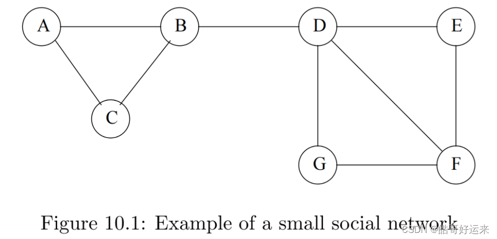
There are many examples of social networks other than “friends” networks. Here, let us enumerate some of the other examples of networks that also exhibit locality of relationships.
Telephone Networks
Here the nodes represent phone numbers, which are really individuals. There is an edge between two nodes if a call has been placed between those phones in some fixed period of time, such as last month, or “ever.” The edges could be weighted by the number of calls made between these phones during the period. Communities in a telephone network will form from groups of people that communicate frequently: groups of friends, members of a club, or people working at the same company, for example.
Email Networks
The nodes represent email addresses, which are again individuals. An edge represents the fact that there was at least one email in at least one direction between the two addresses. Alternatively, we may only place an edge if there were emails in both directions. In that way, we avoid viewing spammers as “friends” with all their victims. Another approach is to label edges as weak or strong. Strong edges represent communication in both directions, while weak edges indicate that the communication was in one direction only. The communities seen in email networks come from the same sorts of groupings we mentioned in connection with telephone networks. A similar sort of network involves people who text other people through their cell phones.
Collaboration Networks
Nodes represent individuals who have published research papers. There is an edge between two individuals who published one or more papers jointly. Optionally, we can label edges by the number of joint publications. The communities in this network are authors working on a particular topic.
An alternative view of the same data is as a graph in which the nodes are papers. Two papers are connected by an edge if they have at least one author in common. Now, we form communities that are collections of papers on the same topic.
There are several other kinds of data that form two networks in a similar way. For example, we can look at the people who edit Wikipedia articles and the articles that they edit. Two editors are connected if they have edited an article in common. The communities are groups of editors that are interested in the same subject. Dually, we can build a network of articles, and connect
articles if they have been edited by the same person. Here, we get communities of articles on similar or related subjects.
In fact, the data involved in Collaborative filtering, as was discussed in Chapter 9, often can be viewed as forming a pair of networks, one for the customers and one for the products. Customers who buy the same sorts of products, e.g., science-fiction books, will form communities, and dually, products that are bought by the same customers will form communities, e.g., all science-fiction books.
Other Examples of Social Graphs
Many other phenomena give rise to graphs that look something like social graphs, especially exhibiting locality. Examples include: information networks (documents, web graphs, patents), infrastructure networks (roads, planes, water pipes, powergrids), biological networks (genes, proteins, food-webs of animals eating each other), as well as other types, like product co-purchasing networks (e.g., Groupon).
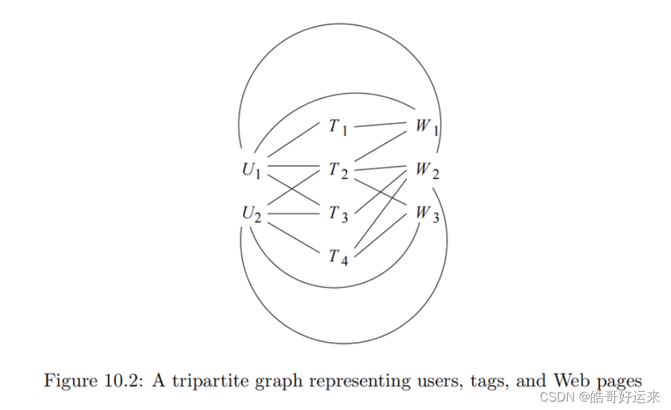
Figure 10.2 is an example of a tripartite graph (the case k = 3 of a k-partite graph). There are three sets of nodes, which we may think of as users { U 1 , U 2 } \{U_1, U_2\} {U1,U2}, tags { T 1 , T 2 , T 3 , T 4 } \{T_1, T_2, T_3, T_4\} {T1,T2,T3,T4}, and Web pages { W 1 , W 2 , W 3 } \{W_1, W_2, W_3\} {W1,W2,W3}.
 Define the betweenness of an edge ( a , b ) (a, b) (a,b) to be the number of pairs of nodes x x x and y y y such that the edge ( a , b ) (a, b) (a,b) lies on the shortest path between x x x and y y y. To be more precise, since there can be several shortest paths between x x x and y y y, edge ( a , b ) (a, b) (a,b) is credited with the fraction of those shortest paths that include the edge ( a , b ) (a, b) (a,b). As in golf, a high score is bad. It suggests that the edge ( a , b ) (a, b) (a,b) runs between two different communities; that is, a a a and b b b do not belong to the same community.
Following is Girvan-Newman Algorithm
Can see this blog: Girvan-Newman Algorithm
A proper definition of a “good” cut must balance the size of the cut itself against the difference in the sizes of the sets that the cut creates. One choice that serves well is the “normalized cut.” First, define the volume of a set S of nodes, denoted V o l ( S ) Vol(S) Vol(S), to be the number of edges with at least one end in S. Suppose we partition the nodes of a graph into two disjoint sets S and T .
Let C u t ( S , T ) Cut(S,T) Cut(S,T) be the number of edges that connect a node in S to a node in T . Then the normalized cut value for S and T is
C u t ( S , T ) V o l ( S ) + C u t ( S , T ) V o l ( T ) \frac{Cut(S,T)}{Vol(S)}+\frac{Cut(S,T)}{Vol(T)} Vol(S)Cut(S,T)+Vol(T)Cut(S,T)
Suppose our graph has adjacency matrix A and degree matrix D. Our third matrix, called the Laplacian matrix, is L = D − A L = D − A L=D−A, the difference between the degree matrix and the adjacency matrix. That is, the Laplacian matrix L has the same entries as D on the diagonal. Off the diagonal, at row i and column j, L has −1 if there is an edge between nodes i and j and 0 if not.
Eigenvalues of the Laplacian Matrix
The smallest eigenvalue for every Laplacian matrix is 0, and its corresponding eigenvector is [1, 1, . . . , 1].
There is a simple way to find the second-smallest eigenvalue for any matrix, such as the Laplacian matrix, that is symmetric (the entry in row i i i and column
j j j equals the entry in row j j j and column i i i). While we shall not prove this fact, the second-smallest eigenvalue of L is the minimum of x T L x x^TLx xTLx, where x = [ x 1 , x 2 , . . . , x n ] x = [x_1, x_2, . . . , x_n] x=[x1,x2,...,xn] is a column vector with n components, and the minimum is
taken under the constraints:
- The length of x is 1; that is ∑ i = 1 n x i 2 = 1 \sum_{i=1}^{n}x_i^2=1 ∑i=1nxi2=1
- x x x is orthogonal to the eigenvector associated with the smallest eigenvalue.
When L is a Laplacian matrix for an n-node graph, we know something more. The eigenvector associated with the smallest eigenvalue is 1. Thus, if x is orthogonal to 1, we must have
x T 1 = ∑ i = 1 n x i = 0 \bold{x}^T\bold{1}=\sum_{i=1}^nx_i=0 xT1=i=1∑nxi=0
In addition for the Laplacian matrix, the expression x T L x x^TLx xTLx has a useful equivalent expression. Recall that L = D − A L = D − A L=D−A, where D and A are the degree and adjacency matrices of the same graph. Thus, x T L x = x T D x − x T A x x^TLx = x^TDx − x^TAx xTLx=xTDx−xTAx.
The Affiliation-Graph Model
The elements of the graph-generation mechanism are:
- There is a given number of communities, and there is a given number of individuals (nodes of the graph).
- Each community can have any set of individuals as members. That is, the memberships in the communities are parameters of the model.
- Each community C has a probability p C p_C pC associated with it, the probability that two members of community C are connected by an edge because they are both members of C. These probabilities are also parameters of the model.
- If a pair of nodes is in two or more communities, then there is an edge between them if any of the communities of which both are members induces that edge according to Rule (3).
- The decision whether a community induces an edge between two of its members is independent of that decision for any other community of which these two individuals are also members.
There is a solution to the problem caused by the affiliation-graph model, where membership of individuals in communities is discrete: either you are a member of the community or not. Instead of “all-or-nothing” membership of nodes in communities, we can suppose that for each node and each community, there is a “strength of membership” for that node and community. Intuitively, the stronger the membership of two individuals in the same community is, the more likely it is that this community will cause there to be an edge between them.
In this model, we can adjust the strength of membership for an individual in a community continuously, just as we can adjust the probability associated with a community in the affiliation-graph model. That improvement allows us to use methods for optimizing continuous functions, such as gradient descent, to maximize the expression for likelihood. In the new model, we have
-
Fixed sets of communities and individuals, as before.
-
For each community C and individual x, there is a strength of membership
parameter F x C F_{xC} FxC . These parameters can take any nonnegative value, and a value of 0 means the individual is definitely not in the community. -
The probability that community C causes there to be an edge between nodes u and v is
p C ( u , v ) = 1 − e − F u C F v C p_C(u,v)=1-e^{-F_{uC}F_{vC}} pC(u,v)=1−e−FuCFvC
As before, the probability of there being an edge between u and v is 1 minus the probability that none of the communities causes there to be an edge between them. That is, each community independently causes edges, and an edge exists between two nodes if any community causes it to exist. More formally, p u v p_{uv} puv, the probability of an edge between nodes u and v, is
p u v = 1 − ∏ C ( 1 − p C ( u , v ) ) p_{uv}=1-\prod_C(1-p_C(u,v)) puv=1−C∏(1−pC(u,v))
Finally, let E be the set of edges in the observed graph. As before, we can write the formula for the likelihood of the observed graph as the product of the expression for p u v p_{uv} puv for each edge ( u , v ) (u, v) (u,v) that is in E, times the product of 1 − p u v 1−p_{uv} 1−puv for each edge ( u , v ) (u, v) (u,v) that is not in E. Thus, in the new model, the formula for the likelihood of the graph with edges E is
∏ ( u , v ) i n E ( 1 − e − F u C F v C ) ∏ ( u , v ) n o t i n E ( e − F u C F v C ) \prod_{(u,v)\space in \space E}(1-e^{-F_{uC}F_{vC}})\prod_{(u,v)\space not\space in \space E}(e^{-F_{uC}F_{vC}}) (u,v) in E∏(1−e−FuCFvC)(u,v) not in E∏(e−FuCFvC)
💡 Continuous Versus Discrete Optimization
Whenever you are trying to find an optimum solution to a problem where some of the elements are continuous (e.g., the probabilities of communities inducing edges) and some elements are discrete (e.g., the memberships of the communities), it might make sense to replace each discrete element by a continuous variable. That change, while it doesn’t strictly speaking represent reality, enables us to perform only one optimization, which will use a continuous optimization method such as gradient descent. We run the risk of winding up in a local optimum that is not the globally best solution.
SimRank
In this section, we shall take up another approach to analyzing social-network graphs. This technique, called “simrank,” applies best to graphs with several types of nodes, although it can in principle be applied to any graph. The purpose of simrank is to measure the similarity between nodes of the same type, and it does so by seeing where random walkers on the graph wind up when starting at a particular node, the source node. Because calculation must be carried out once for each source node, there is a limit to the size of graphs that can be analyzed completely in this manner. However, we shall also offer an algorithm that approximates simrank, but is far more efficient than iterated matrix-vector multiplication. Finally, we show how simrank can be used to find communities.
Let us use β as the probability that the walker continues at random, so 1 − β is the probability the walker will teleport to the source node S. Let e S e_S eS be the column vector that has 1 in the row for node S and 0’s elsewhere. Then if v is the column vector that reflects the probability the walker is at each of the nodes at a particular round, and v ′ v′ v′ is the probability the walker is at each of the nodes at the next round, then v ′ v′ v′ is related to v by:
v ′ = β M v + ( 1 − β ) e S v'=\beta Mv+(1-\beta)e_S v′=βMv+(1−β)eS
A simple approach is to add nodes until the density of edges – the fraction of edges that connect nodes in the community divided by the number of possible edges connecting nodes in the community (i.e., C 2 n C_2^n C2n for an n-node community) – goes below a threshold.
Another measure of the goodness of a community C is the conductance. To define conductance, we need first to define the volume of a community C, which is the smaller of the sum of the degrees of the nodes in C and the sum of the degrees of the nodes not in C. Then the conductance of C is the ratio of the number of edges with exactly one end in C divided by the volume of C. The intuitive idea behind conductance is that it looks for sets C that are neither too small nor too large, and yet can be disconnected from the network by cutting a relatively small number of edges. Small conductance suggests a closely knit community.
The neighborhood of radius d for a node v is the set of nodes u for which there is a path of length at most d from v to u. We denote this neighborhood by N ( v , d ) N(v, d) N(v,d). For example, N(v, 0) is always {v}, and N(v, 1) is v plus the set of nodes to which there is an arc from v. More generally, if V is a set of nodes, then N(V, d) is the set of nodes u for which there is a path of length d or less from at least one node in the set V .
The neighborhood profile of a node v is the sequence of sizes of its neighborhoods ∣ N ( v , 1 ) ∣ , ∣ N ( v , 2 ) ∣ , . . . . |N(v, 1)|, |N(v, 2)|, . . . . ∣N(v,1)∣,∣N(v,2)∣,.... We do not include the neighborhood of distance 0, since its size is always 1.
Summary of Chapter 10
- Social-Network Graphs: Graphs that represent the connections in a social network are not only large, but they exhibit a form of locality, where small subsets of nodes (communities) have a much higher density of edges than the average density.
- Communities and Clusters: While communities resemble clusters in some ways, there are also significant differences. Individuals (nodes) normally belong to several communities, and the usual distance measures fail to represent closeness among nodes of a community. As a result, standard algorithms for finding clusters in data do not work well for community finding.
- Betweenness: One way to separate nodes into communities is to measure the betweenness of edges, which is the sum over all pairs of nodes of the fraction of shortest paths between those nodes that go through the given edge. Communities are formed by deleting the edges whose betweenness is above a given threshold.
- The Girvan-Newman Algorithm: The Girvan-Newman Algorithm is an efficient technique for computing the betweenness of edges. A breadth-first search from each node is performed, and a sequence of labeling steps computes the share of paths from the root to each other node that go through each of the edges. The shares for an edge that are computed for each root are summed to get the betweenness.
- Communities and Complete Bipartite Graphs: A complete bipartite graph has two groups of nodes, all possible edges between pairs of nodes chosen one from each group, and no edges between nodes of the same group. Any sufficiently dense community (a set of nodes with many edges among them) will have a large complete bipartite graph.
- Finding Complete Bipartite Graphs: We can find complete bipartite graphs by the same techniques we used for finding frequent itemsets. Nodes of the graph can be thought of both as the items and as the baskets. The basket corresponding to a node is the set of adjacent nodes, thought of as items. A complete bipartite graph with node groups of size t and s can be thought of as finding frequent itemsets of size t with supports.
- Graph Partitioning: One way to find communities is to partition a graph repeatedly into pieces of roughly similar sizes. A cut is a partition of the nodes of the graph into two sets, and its size is the number of edges that have one end in each set. The volume of a set of nodes is the number of edges with at least one end in that set.
- Normalized Cuts: We can normalize the size of a cut by taking the ratio of the size of the cut and the volume of each of the two sets formed by the cut. Then add these two ratios to get the normalized cut value. Normalized cuts with a low sum are good, in the sense that they tend to divide the nodes into two roughly equal parts, and have a relatively small size.
- Adjacency Matrices: These matrices describe a graph. The entry in row i and column j is 1 if there is an edge between nodes i and j, and 0 otherwise.
- Degree Matrices: The degree matrix for a graph has d in the ith diagonal entry if d is the degree of the ith node. Off the diagonal, all entries are 0.
- Laplacian Matrices: The Laplacian matrix for a graph is its degree matrix minus its adjacency matrix. That is, the entry in row i and column i of the Laplacian matrix is the degree of the ith node of the graph, and the entry in row i and column j, for i 6 = j, is −1 if there is an edge between nodes i and j, and 0 otherwise.
- Spectral Method for Partitioning Graphs: The lowest eigenvalue for any Laplacian matrix is 0, and its corresponding eigenvector consists of all 1’s. The eigenvectors corresponding to small eigenvalues can be used to guide a partition of the graph into two parts of similar size with a small cut value. For one example, putting the nodes with a positive component in the eigenvector with the second-smallest eigenvalue into one set and those with a negative component into the other is usually good.
- Overlapping Communities: Typically, individuals are members of several communities. In graphs describing social networks, it is normal for the probability that two individuals are friends to rise as the number of communities of which both are members grows.
- The Affiliation-Graph Model: An appropriate model for membership in communities is to assume that for each community there is a probability that because of this community two members become friends (have an edge in the social network graph). Thus, the probability that two nodes have an edge is 1 minus the product of the probabilities that none of the communities of which both are members cause there to be an edge between them. We then find the assignment of nodes to communities and the values of those probabilities that best describes the observed social graph.
- Maximum-Likelihood Estimation: An important modeling technique, useful for modeling communities as well as many other things, is to compute, as a function of all choices of parameter values that the model allows, the probability that the observed data would be generated. The values that yield the highest probability are assumed to be correct, and called the maximum-likelihood estimate (MLE).
- Use of Gradient Descent: If we know membership in communities, we can find the MLE by gradient descent or other methods. However, we cannot find the best membership in communities by gradient descent, because membership is discrete, not continuous.
- Improved Community Modeling by Strength of Membership: We can formulate the problem of finding the MLE of communities in a social graph by assuming individuals have a strength of membership in each community, possibly 0 if they are not a member. If we define the probability of an edge between two nodes to be a function of their membership strengths in their common communities, we can turn the problem of finding the MLE into a continuous problem and solve it using gradient descent.
- Simrank: One way to measure the similarity of nodes in a graph with several types of nodes is to start a random walker at one node and allow it to wander, with a fixed probability of restarting at the same node. The distribution of where the walker can be expected to be is a good measure of the similarity of nodes to the starting node. This process must be repeated with each node as the starting node if we are to get all-pairs similarity.
- Triangles in Social Networks: The number of triangles per node is an important measure of the closeness of a community and often reflects its maturity. We can enumerate or count the triangles in a graph with m edges in O ( m 3 / 2 ) O(m^{3/2}) O(m3/2) time, but no more efficient algorithm exists in general.
- Triangle Finding by MapReduce: We can find triangles in a single round of MapReduce by treating it as a three-way join. Each edge must be sent to a number of reducers proportional to the cube root of the total number of reducers, and the total computation time spent at all the reducers is proportional to the time of the serial algorithm for triangle finding.
- Neighborhoods: The neighborhood of radius d for a node v in a directed or undirected graph is the set of nodes reachable from v along paths of length at most d. The neighborhood profile of a node is the sequence of neighborhood sizes for all distances from 1 upwards. The diameter of a connected graph is the smallest d for which the neighborhood of radius d for any starting node includes the entire graph.
- Transitive Closure: A node v can reach node u if u is in the neighborhood of v for some radius. The transitive closure of a graph is the set of pairs of nodes (v, u) such that v can reach u.
- Computing Transitive Closure: Since the transitive closure can have a number of facts equal to the square of the number of nodes of a graph, it is infeasible to compute transitive closure directly for large graphs. One approach is to find strongly connected components of the graph and collapse them each to a single node before computing the transitive closure.
- Transitive Closure and MapReduce: We can view transitive closure computation as the iterative join of a path relation (pairs of nodes v and u such that u is known to be reachable from v) and the arc relation of the graph. Such an approach requires a number of MapReduce rounds equal to the diameter of the graph.
- Seminaive Evaluation: When computing the transitive closure for a graph, we can speed up the iterative evaluation of the Path relation by recognizing that a Path fact is only useful on the round after that round when it was first discovered. A similar idea speeds up the reachability calculation and many similar iterative algorithms.
- Transitive Closure by Recursive Doubling: An approach that uses fewer MapReduce rounds is to join the path relation with itself at each round. At each round, we double the length of paths that are able to contribute to the transitive closure. Thus, the number of needed rounds is only the base-2 logarithm of the diameter of the graph.
- Smart Transitive Closure: While recursive doubling can cause the same path to be considered many times, and thus increases the total computation time (compared with iteratively joining paths with single arcs), a variant called smart transitive closure avoids discovering the same path more than once. The trick is to require that when joining two paths, the first has a length that is a power of 2.
- Approximating Neighborhood Sizes: By using the Flajolet-Martin technique for approximating the number of distinct elements in a stream, we can find the neighborhood sizes at different radii approximately. We maintain a set of tail lengths for each node. To increase the radius by 1, we examine each edge (u, v) and for each tail length for u we set it equal to the corresponding tail length for v if the latter is larger than the former.
相关文章:

斯坦福数据挖掘教程·第三版》读书笔记(英文版)Chapter 10 Mining Social-Network Graphs
来源:《斯坦福数据挖掘教程第三版》对应的公开英文书和PPT。 Chapter 10 Mining Social-Network Graphs The essential characteristics of a social network are: There is a collection of entities that participate in the network. Typically, these entiti…...

DFS:842. 排列数字
给定一个整数 nn,将数字 1∼n1∼n 排成一排,将会有很多种排列方法。 现在,请你按照字典序将所有的排列方法输出。 输入格式 共一行,包含一个整数 nn。 输出格式 按字典序输出所有排列方案,每个方案占一行。 数据…...
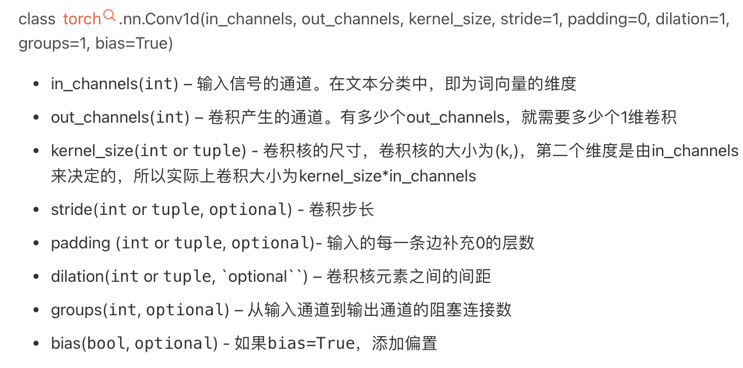
pytorch之nn.Conv1d详解
自然语言处理中一个句子序列,一维的,所以使用Conv1d...

H5生成二维码
H5生成二维码: 1.引入js库,可自行点击链接复制使用 <script type"text/javascript" src"http://static.runoob.com/assets/qrcode/qrcode.min.js"></script>2.加入二维码占位区HTML <div id"qrCode">…...

Three.js加载360全景图片/视频
Three.js加载360全景图片/视频 效果 原理 将全景图片/视频作为texture引入到three.js场景中将贴图与球形网格模型融合,将球模型当做成环境容器使用处理视频时需要以dom为载体,加载与控制视频动作每次渲染时更新当前texture,以达到视频播放效…...

北大硕士7年嵌入式学习经验分享
阶段 1 大一到大三这个阶段我与大多数学生相同: 学习本专业知识(EE专业),学习嵌入式软件开发需要的计算机课程(汇编原理,计算机组成原理,操作系统,C语言等),…...

华为鸿蒙手表开发之动态生成二维码
华为鸿蒙手表开发之动态生成二维码 前言: 最近入职新公司,由于之前的哥们临时离职,走得很突然,所以没有任何交接和文档,临时顶上公司手表应用的上架,更换了新的密钥和key之后重新测试功能和流程ÿ…...
2023-09-28 monetdb-databae的概念和作用-分析
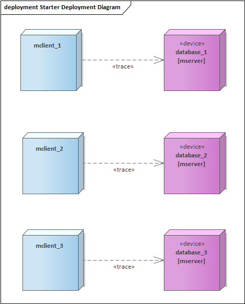
摘要: 每个数据库对于db,schema以及user,role都有一套自己的设计, 不同数据库间对于相同名字的东西例如database和schema可以说南辕北辙, 例如mysql中schema其实是database的同义词. 本文分析monetdb的database的概念和作用 database的概念和作用: 和mysql的database完全不同…...
2024级199管理类联考之数学基础(上篇)
管理类考试介绍 管理综合200分,时间3小时 数学:75分/25题,是拉开差距的核心模块 问题求解题:15个,5选一条件充分性判断:10个,结合两个条件选择答案 条件一充分,条件二不充分:A条件一不充分,条件二充分:B条件一充分,条…...

RFID技术引领汽车零部件加工新时代
RFID技术的兴起引领了汽车零部件加工领域的新时代,作为一种利用无线电频率进行自动识别的技术,RFID技术能够快速、准确地识别物体并获取相关数据,在汽车零部件加工中,RFID技术具有重要的应用价值,可以提高生产效率、降…...
python中使用matplotlib绘图
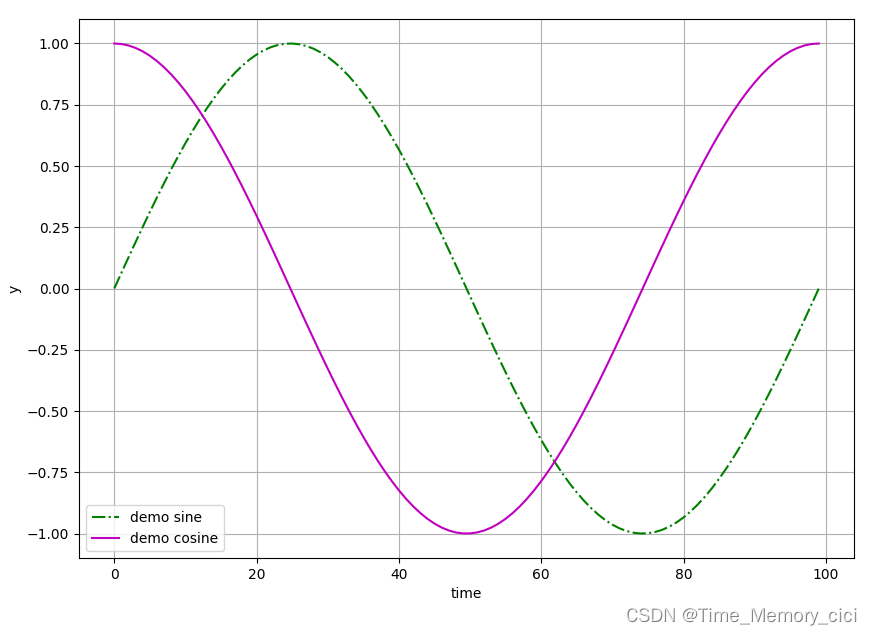
一、背景 当我们在写python程序时,不可避免的需要将数据可视化,也就是绘制出数据的曲线图,以便我们更直观的观察数据间的变化,和方便对比。此时就要用到matplotlib库了。 matplotlib官方给出的定义是: 翻译过来也就是…...

Qt Creator 使用技巧
使用技巧 功能快捷键解释Switch Header/SourceF4在同名的头文件和源程序文件之间切换Follow Symbol Under CursorF2变量:跳转到声明;函数:声明和定义切换Refactor Rename Symbol Under CursorCtrlShiftR改名称,将替换所有用到这个符号的地方RefactorAdd Definition…...

来看看双阶段目标检测算法趴
🚀 作者 :“码上有钱” 🚀 文章简介 :AI-目标检测算法 🚀 欢迎小伙伴们 点赞👍、收藏⭐、留言💬简介 双阶段目标检测算法是一类深度学习算法,通常分为两个阶段来检测和识别图像中的…...
python利用matplotlib绘图,对于中文和负号不显示,显示方框“口口”完美解决办法!!
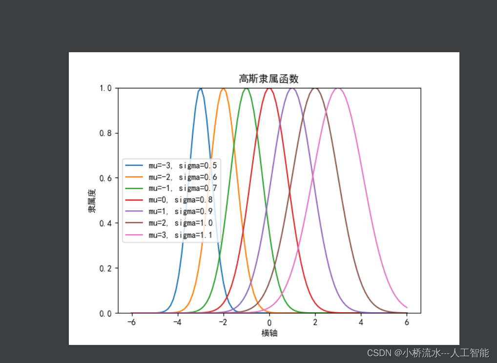
文章目录 一、问题展示二、问题分析三、解决办法四、结果展示 一、问题展示 二、问题分析 可以发现对中文,以及负号不显示。 三、解决办法 import matplotlib.pyplot as pltplt.rcParams[font.sans-serif] [usimHei] # 显示中文 plt.rcParams[axes.unicode_mi…...
【数组及指针经典笔试题解析】
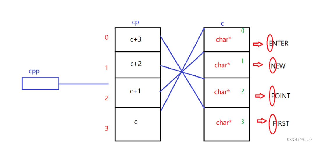
1.数组和指针笔试题 题目1 int main(){int a[5] { 1,2,3,4,5};int * ptr (int * )(&a 1);printf("%d,%d",*(a 1),*(ptr - 1));return 0;}图文解析: int * ptr …...
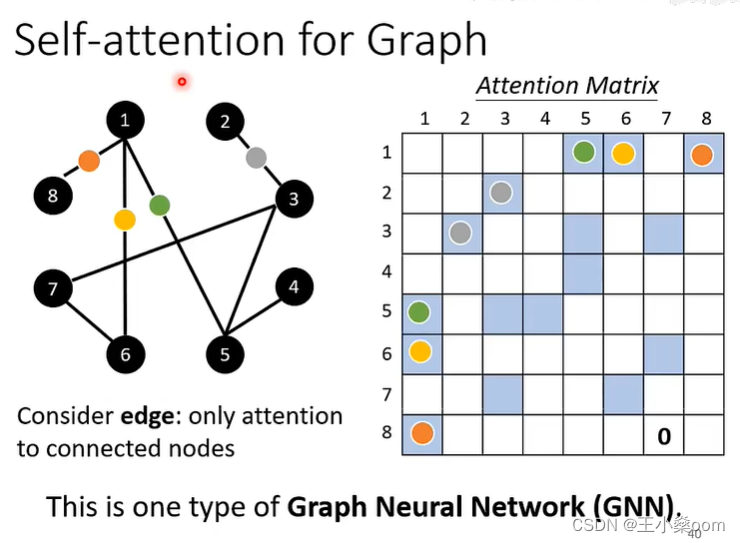
Transformer学习-self-attention
这里写自定义目录标题 Self-attentionMulti-head self-attention用self-attention解决其他问题 Self-attention 用Wq、Wk、Wv分别乘输入向量得到q、k、v向量 用每个q向量乘所有的k向量得到对应项的attention,即用每项的query向量去匹配所有的key向量,得…...

Spring Boot:利用JPA进行数据库的增改
目录 JPA介绍Service接口Service和Autowired示例代码 Dao数据库操作层Repository示例代码 控制器文件示例代码-增加增加成功示例代码-修改修改成功 JPA介绍 JPA(Javaa Persistence API)一种用于持久化 Java 对象到关系型数据库的标准规范。它提供了一种统一的方式来…...
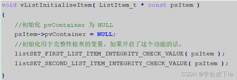
列表的增删改查和遍历
任务概念 什么是任务 任务是一个参数为指针,无法返回的函数,函数体为死循环不能返回任务的实现过程 每个任务是独立的,需要为任务分别分配栈称为任务栈,通常是预定义的全局数组,也可以是动态分配的一段内存空间&#…...

获取网卡上的IP、网关及DNS信息,获取最佳路由,遍历路由表中的条目(附源码)
VC常用功能开发汇总(专栏文章列表,欢迎订阅,持续更新...)https://blog.csdn.net/chenlycly/article/details/124272585C软件异常排查从入门到精通系列教程(专栏文章列表,欢迎订阅,持续更新...&a…...
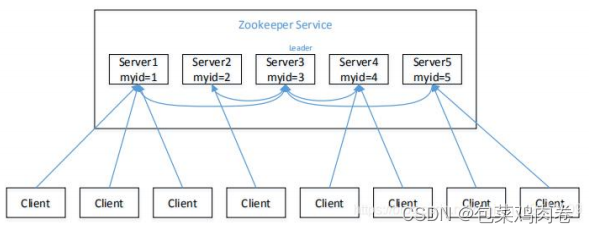
保姆级 -- Zookeeper超详解
1. Zookeeper 是什么(了解) Zookeeper 是一个 分布式协调服务 的开源框架, 主要用来解决分布式集群中应用系统的一致性问题, 例如怎样避免同时操作同一数据造成脏读的问题. ZooKeeper 本质上是 一个分布式的小文件存储系统 . 提供基于类似于文件系统的目录树方式的数据存储, …...

基于SQL数据库的酒店管理系统
一、数据库设计 1.需求分析 客房的预定:可以通过网络进行预定,预定修改,取消预订。 客房管理:预定管理、客房查询、设置房态、开房、换房、续住、退房等管理。 员工管理: 员工修改信息、人员调配。 账务管理࿱…...

基于微信小程序的大学生租房平台[小程序]-计算机毕业设计源码+LW文档
摘要:随着高校学生数量的增加,大学生租房需求日益增长。为解决大学生租房过程中信息不对称、流程繁琐等问题,本文设计并实现了一个基于微信小程序的大学生租房平台。该平台涵盖系统用户管理、新闻数据管理、房源管理、预约看房管理、合同管理…...

java快速排序超详细总结:核心实现+简化版+趣味版
java快速排序超详细总结:核心实现简化版趣味版面试高频 | 四种写法 | 含过程演示 | 新手友好概要 详解快速排序三种写法:挖坑法、双指针交换法、单指针法,每种均附分步演示与代码注释。涵盖复杂度分析、稳定性及面试易错点,附Pyth…...

Course15:视觉大模型与多模态理解
Qwen 多模态模型中图片 Token ID 与向量的核心理解文本 Token 是 “语言的最小语义单元”,图片 Token 是 “视觉的最小特征单元”—— 两者最终都会被映射到同一维度的向量空间,让模型能 “读懂” 图文的关联语义。维度文本 Token(如 Qwen 的…...

干货来了:本科生专属降AI率平台,千笔·专业降AI率智能体 VS 锐智 AI
在AI技术迅速发展的今天,越来越多的本科生开始借助AI工具辅助论文写作,以提高效率、优化内容。然而,随着学术审核标准日益严格,AI生成内容的痕迹越来越容易被检测出来,导致论文AI率超标成为普遍难题。许多学生在反复修…...

使用MATLAB进行SUNFLOWER MATCH LAB模型输出结果的可视化分析
使用MATLAB进行SUNFLOWER MATCH LAB模型输出结果的可视化分析 对于很多科研工作者和数据分析师来说,MATLAB是一个再熟悉不过的老朋友了。它强大的矩阵运算能力和丰富的可视化工具箱,让数据分析和结果呈现变得得心应手。然而,当我们使用像SUN…...

EasyAnimateV5-7b-zh-InP MySQL数据库驱动视频生成系统
EasyAnimateV5-7b-zh-InP MySQL数据库驱动视频生成系统 1. 引言 想象一下,你运营着一个电商平台,每天需要为上千件商品生成展示视频。传统方式需要设计师手动制作,成本高、效率低,而且很难保证风格统一。现在,通过结…...

FireRed-OCR Studio完整指南:FireRed-OCR Studio API服务化封装与FastAPI集成
FireRed-OCR Studio完整指南:FireRed-OCR Studio API服务化封装与FastAPI集成 1. 产品概述 FireRed-OCR Studio是一款基于Qwen3-VL模型开发的工业级文档解析工具,它重新定义了文档数字化的标准。不同于传统OCR工具只能识别文字内容,FireRed…...

VideoAgentTrek-ScreenFilter一文详解:class_id与class_name映射关系说明
VideoAgentTrek-ScreenFilter一文详解:class_id与class_name映射关系说明 在视频和图像分析领域,目标检测模型的核心输出之一就是识别出画面中的物体并对其进行分类。对于开发者而言,理解模型输出的类别标识(class_id)…...

K8S HPA自动扩缩容实战指南
文章目录前言1、简介2、工作原理3、HPA版本变革4、监控指标类型4、HPA配置资源清单4.1 基于CPU负载实现自动扩缩容NAME:这是 HPA 对象的名称REFERENCE:HPA 监控和自动扩展的目标对象。TARGETS:当前和目标的资源使用情况MINPODS:HP…...
