【监控指标】监控系统-prometheus、grafana。容器化部署。go语言 gin框架、gRPC框架的集成
文章目录
- 一、监控有哪些指标
- 二、prometheus、grafana架构
- Prometheus 组件
- Grafana 组件
- 架构优点
- 三、安装prometheus和node-exporter
- 1. docker pull镜像
- 2. 启动node-exporter
- 3. 启动prometheus
- 四、promql基本语法
- 五、grafana的安装和使用
- 1. 新建空文件夹grafana-storage,用来存储数据
- 2. 启动grafana(如果和已有的端口冲突改一下端口)
- 3. 配置prometheus并使用
- 六、导入Grafana模板
- 七、guages、counter、histograms指标
- guages
- Counter
- Histograms
- 八、go语言集成prometheus
- 九、grpc框架集成prometheus
- 十、gin框架集成prometheus
一、监控有哪些指标
监控1. 业务监控(上层概念 - 领导层):需求方:老板、运营开发方: 大数据库 ,都会访问业务库,大数据库会从同步库, 宽表QPS、DAU日活、访问状态(http code)、业务接口(登录、注册、聊天、上传、留言、搜索、投诉)、 产品转换率、充值额度2. 系统监控需求方: 运维开发方: 运维操作系统相关: cpu使用率、内存使用、磁盘使用率、磁盘空间(非常常见)、TCP(上W的链接),流量组件: mysql、redis、kafka3. 日志监控需求方:运维、开发开发方:开发两种日志:业务日志(大数据, 普通日志)、 系统日志(操作系统日志、mysql组件日志、kakfa的日志)监控中的重头戏,一般我们都会对单独针对日志设计日志管理系统, ELK日志系统, loki4. 网络监控:需求方:机房管理开放方:服务器管理IDC 交换机、路由器、防火墙、负载均衡、服务器、机柜、电源、UPS、空调、网络设备、机房环境监控,网络:内部网络(物理内网,虚拟内网(VPN))监控5. 程序监控:需求方:开发开发方:开发比如产生了 500 ErrUserNotFound一般要运维和开发人员配合,开发人员在程序中提供监控接口,运维人员通过接口获取监控数据prometheus的数据格式: metricsmetrics是一种对采样数据的总称二、prometheus、grafana架构
官网:https://prometheus.fuckcloudnative.io/di-yi-zhang-jie-shao/overview
Prometheus 组件
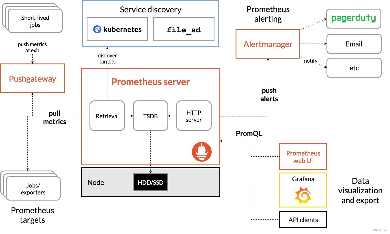
- Prometheus server:Prometheus 的核心组件,负责收集、存储和查询时间序列数据。
- Exporters:Exporters 是 Prometheus 用来从目标系统收集数据的插件。Exporters 可以是主动拉取数据的,也可以是被动推送数据的。
- Pushgateway:Pushgateway 是一个被动推送数据的 Exporter,用于收集短暂运行的任务或服务的数据。
- Alertmanager:Alertmanager 负责处理 Prometheus 发出的告警,并将告警发送到指定的通知系统。
- Prometheus web UI:Prometheus 自带的 Web 界面,用于查看 Prometheus 收集的数据。
Grafana 组件
- Grafana:一个开源的图形化数据可视化工具,用于将 Prometheus 的数据进行可视化展示。
架构说明
Prometheus通过 Exporters 从目标系统收集数据,并将数据存储到 Prometheus server。Prometheus server 还可以通过 Pushgateway 收集短暂运行的任务或服务的数据。Alertmanager 负责处理 Prometheus 发出的告警,并将告警发送到指定的通知系统。Prometheus web UI 用于查看 Prometheus 收集的数据。
Grafana 与 Prometheus 的结合
Grafana 可以与 Prometheus 结合使用,将 Prometheus 的数据进行可视化展示。Grafana 可以创建各种类型的图表,用于展示 Prometheus 的数据,例如曲线图、柱状图、饼图等。
架构优点
Prometheus 和 Grafana 的结合具有以下优点:
- 可扩展性:Prometheus 和 Grafana 都是可扩展的系统,可以满足不同规模的监控需求。
- 灵活性:Prometheus 和 Grafana 提供了丰富的功能,可以满足不同的监控需求。
- 开源:Prometheus 和 Grafana 都是开源软件,可以免费使用。
三、安装prometheus和node-exporter
1. docker pull镜像
docker pull prom/node-exporter
docker pull prom/prometheus
docker pull grafana/grafana
2. 启动node-exporter
docker run -d -p 9100:9100 -v "/proc:/host/proc:ro" -v "/sys:/host/sys:ro" -v "/:/rootfs:ro" prom/node-exporter
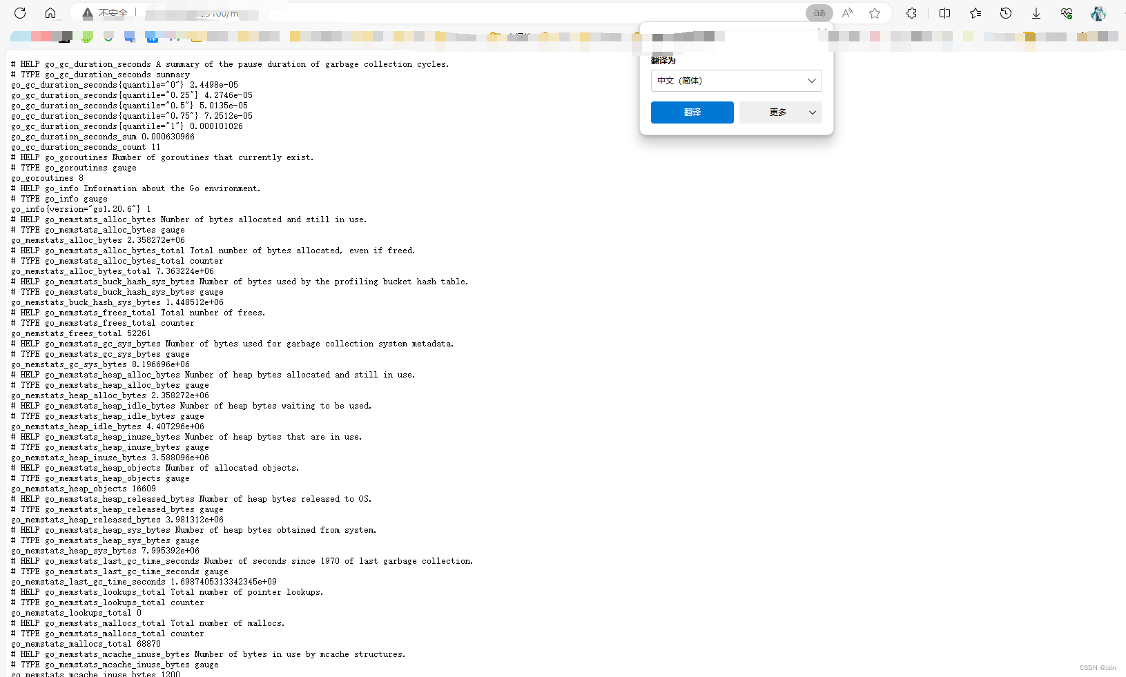
访问url:
http://127.0.0.1:9100/metrics
3. 启动prometheus
建立 /opt/prometheus/prometheus.yml
内容如下:
global:scrape_interval: 60sevaluation_interval: 60sscrape_configs:- job_name: prometheusstatic_configs:- targets: ['localhost:9090']labels:instance: prometheus- job_name: linuxstatic_configs:- targets: ['自己的ip:9100']labels:instance: localhost
启动:
docker run -d \
-p 9090:9090 \
-v /opt/prometheus/prometheus.yml:/etc/prometheus/prometheus.yml \
prom/prometheus
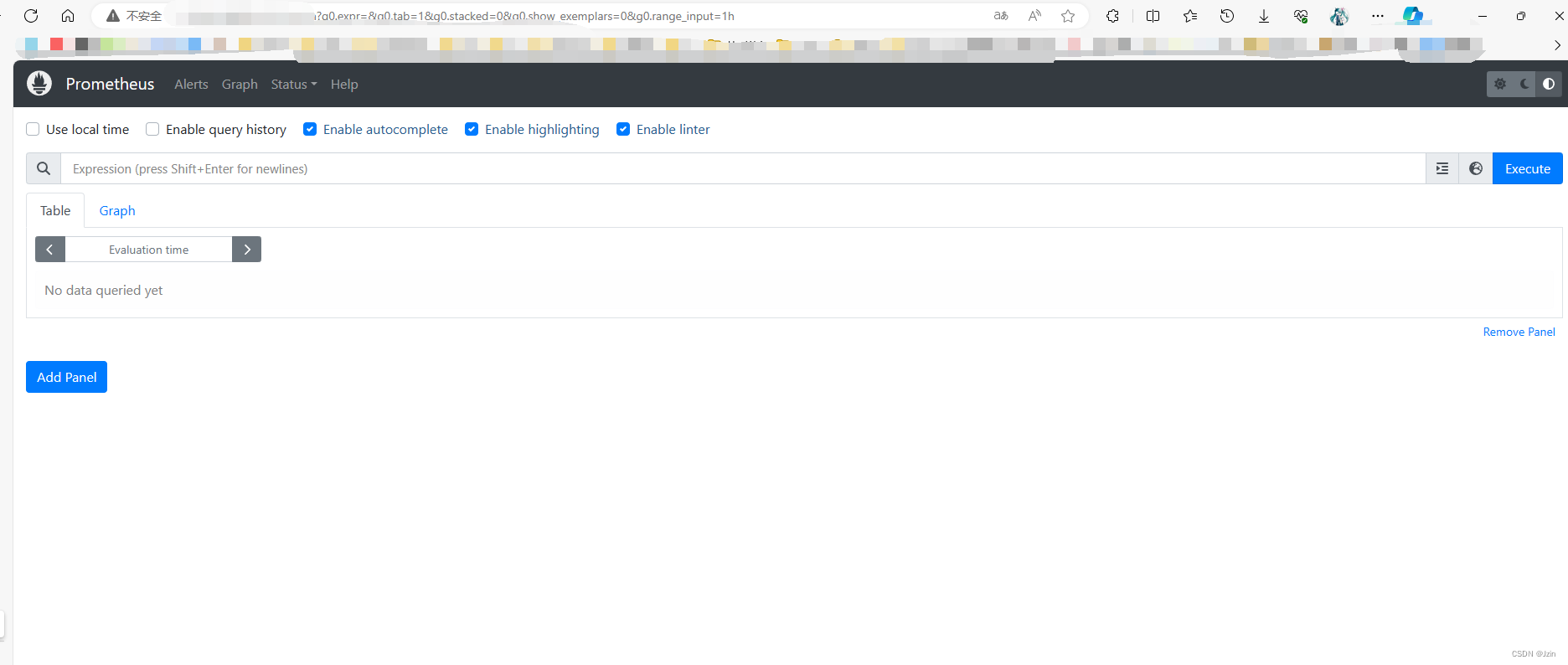
访问url:
127.0.0.1:9090/graph
四、promql基本语法
不需要花过多的精力学习它 用到的时候使用即可
Prometheus Query Language(PromQL)是用于查询和分析从 Prometheus 中收集的监控指标数据的查询语言。以下是 PromQL 的基本语法和一些常见的查询操作符:
-
选择时间范围:
time(): 获取当前时间戳。timestamp(): 将时间戳转换为日期和时间。offset <duration>: 偏移查询的时间范围。
-
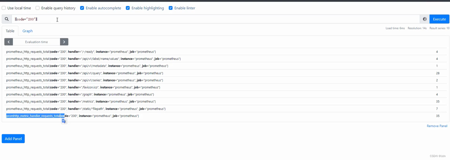
选择指标数据:
<metric_name>: 选择具体的指标名称。{<label_name>=<label_value>}: 使用标签选择指标实例。up{job="api"}: 选择标签job等于api的指标数据。
-
基本查询操作符:
=: 等于。!=: 不等于。=~: 正则表达式匹配。!~: 不匹配正则表达式。
-
聚合操作:
sum(<vector>): 对指标数据进行求和。avg(<vector>): 对指标数据取平均值。min(<vector>): 获取指标数据的最小值。max(<vector>): 获取指标数据的最大值。count(<vector>): 计算指标数据的数量。rate(<vector>[<duration>]): 计算速率,通常用于计算速率指标,例如请求速率。increase(<vector>[<duration>]): 计算增长量,通常用于计算计数器类型的指标。
-
时间窗口:
[<duration>]: 指定查询的时间范围。offset <duration>: 设置查询时间范围的偏移量。
-
聚合函数:
by(<label>): 按标签对结果进行分组。topk(<k>, <vector>): 获取前 k 个结果。quantile(<q>, <vector>): 计算分位数。
-
布尔操作:
and: 逻辑与。or: 逻辑或。unless: 逻辑非。
-
函数:PromQL 支持多种函数,用于对指标数据进行操作和处理,如
abs(),floor(),ceil(),round()等。 -
括号:可以使用括号来控制操作符的优先级。
以下是一些示例 PromQL 查询:
up{job="api"}: 选择标签job等于api的up指标数据。sum(rate(http_requests_total{job="web"}[5m])): 计算过去 5 分钟内job为web的http_requests_total指标的速率总和。node_cpu{mode="idle"} / ignoring(cpu) group_left sum(node_cpu):计算node_cpu中mode为 “idle” 的 CPU 使用率与所有 CPU 使用率的比例,同时按node_cpu的标签进行分组。
PromQL 具有丰富的功能和语法,允许您执行各种复杂的查询和分析操作,以满足您的监控需求。要深入了解 PromQL,请参考 Prometheus 官方文档或相关教程。
五、grafana的安装和使用
1. 新建空文件夹grafana-storage,用来存储数据
mkdir /opt/grafana-storage
chmod 777 -R /opt/grafana-storage
2. 启动grafana(如果和已有的端口冲突改一下端口)
docker run -d -p 3000:3000 --name=grafana -v /opt/grafana-storage/:/var/lib/grafana grafana/grafana
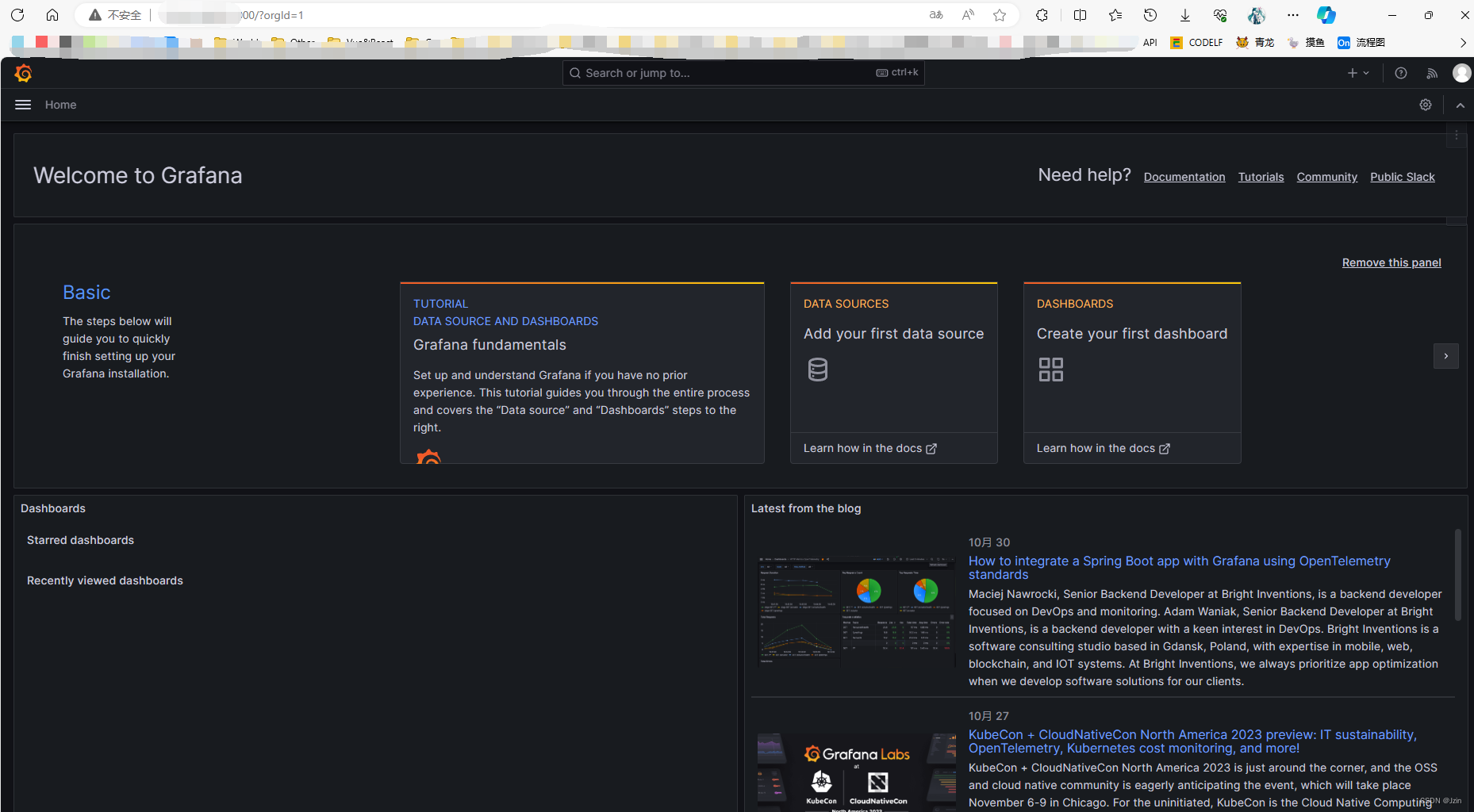
访问:
127.0.0.1:3000
默认用户名密码:admin/admin
3. 配置prometheus并使用
点进Data sources
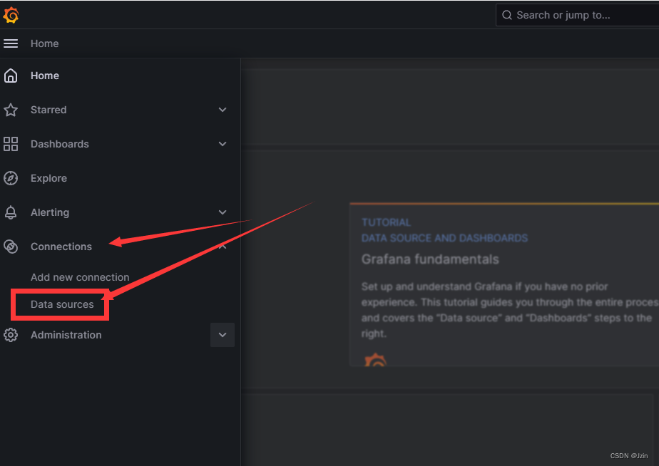
然后add一个
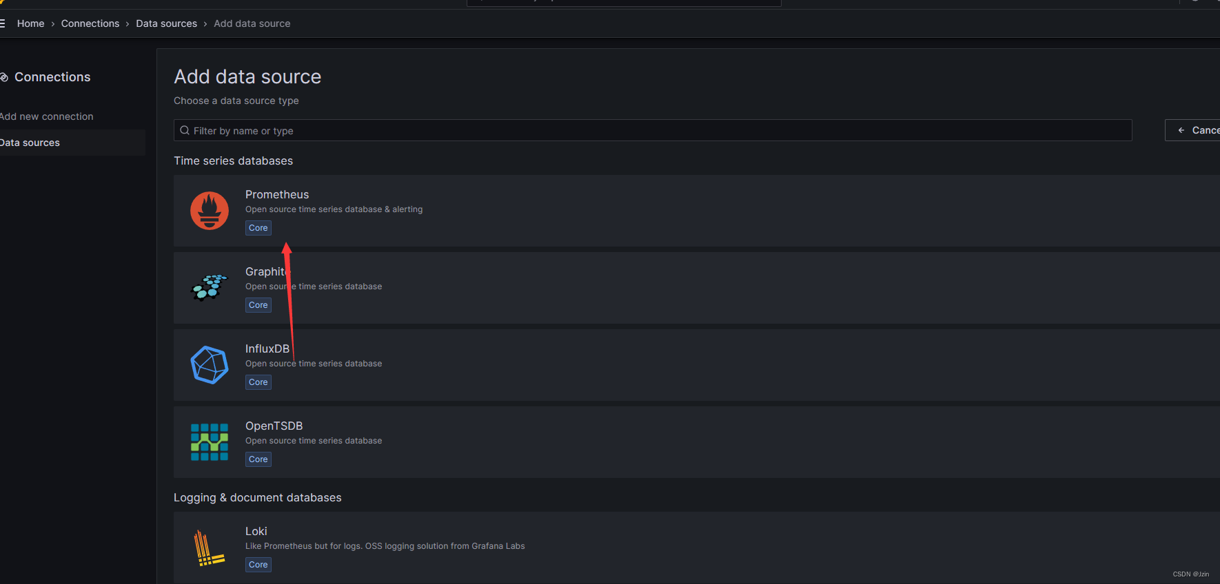
输入自己的ip直接完成:
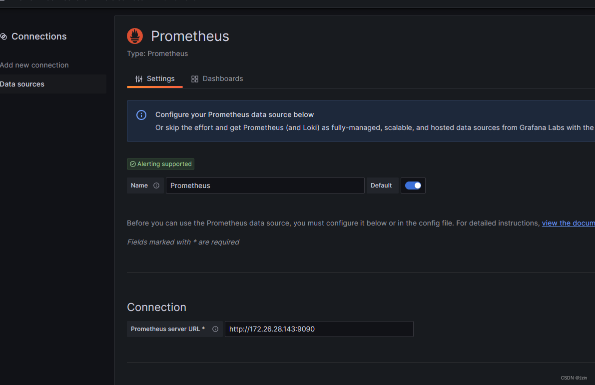
这时候没有展示 展示什么需要自己配置
重点了解一下panel或row就可以了
panel是仪表盘
row是很多panel
这里直接点蓝按钮了
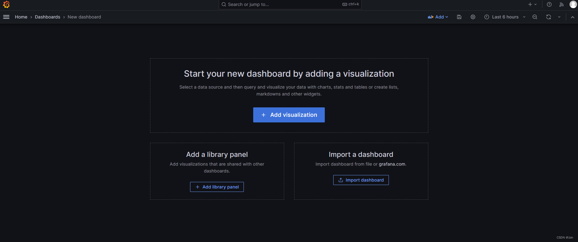
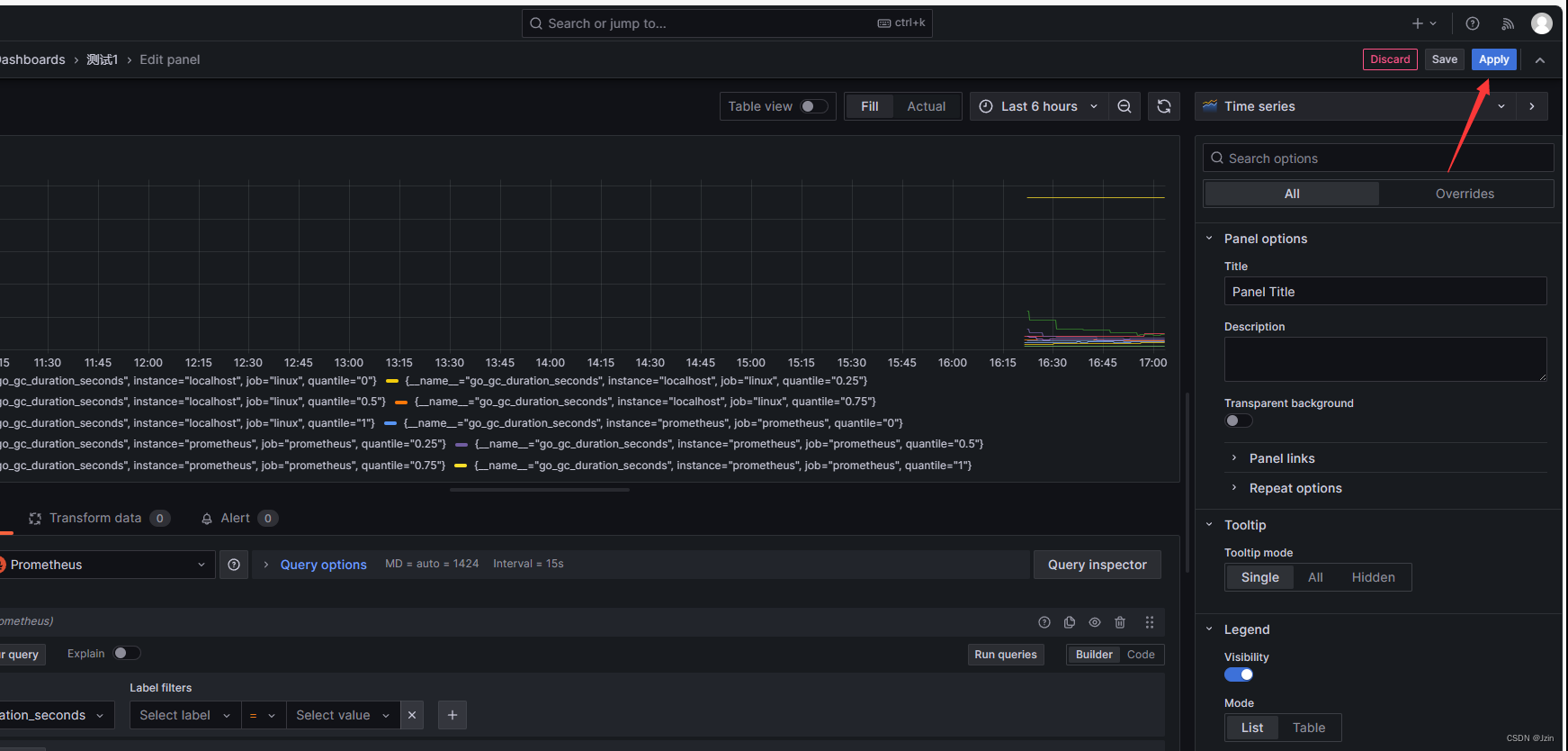
然后进行查询就可以看到数据了
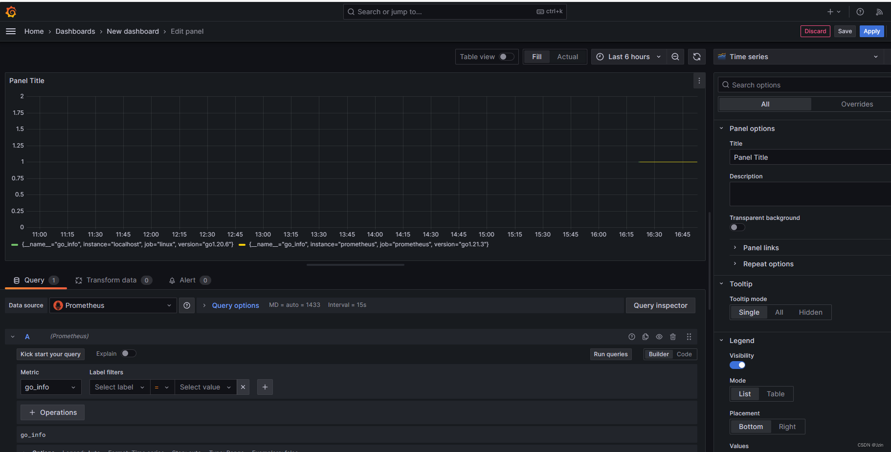
这里apply以后可以save保存
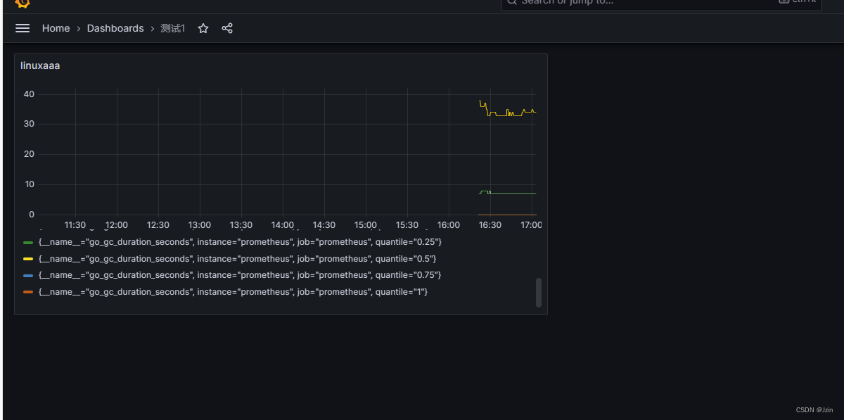
保存完以后可以直接进来看你创建的指标 也就是一个row
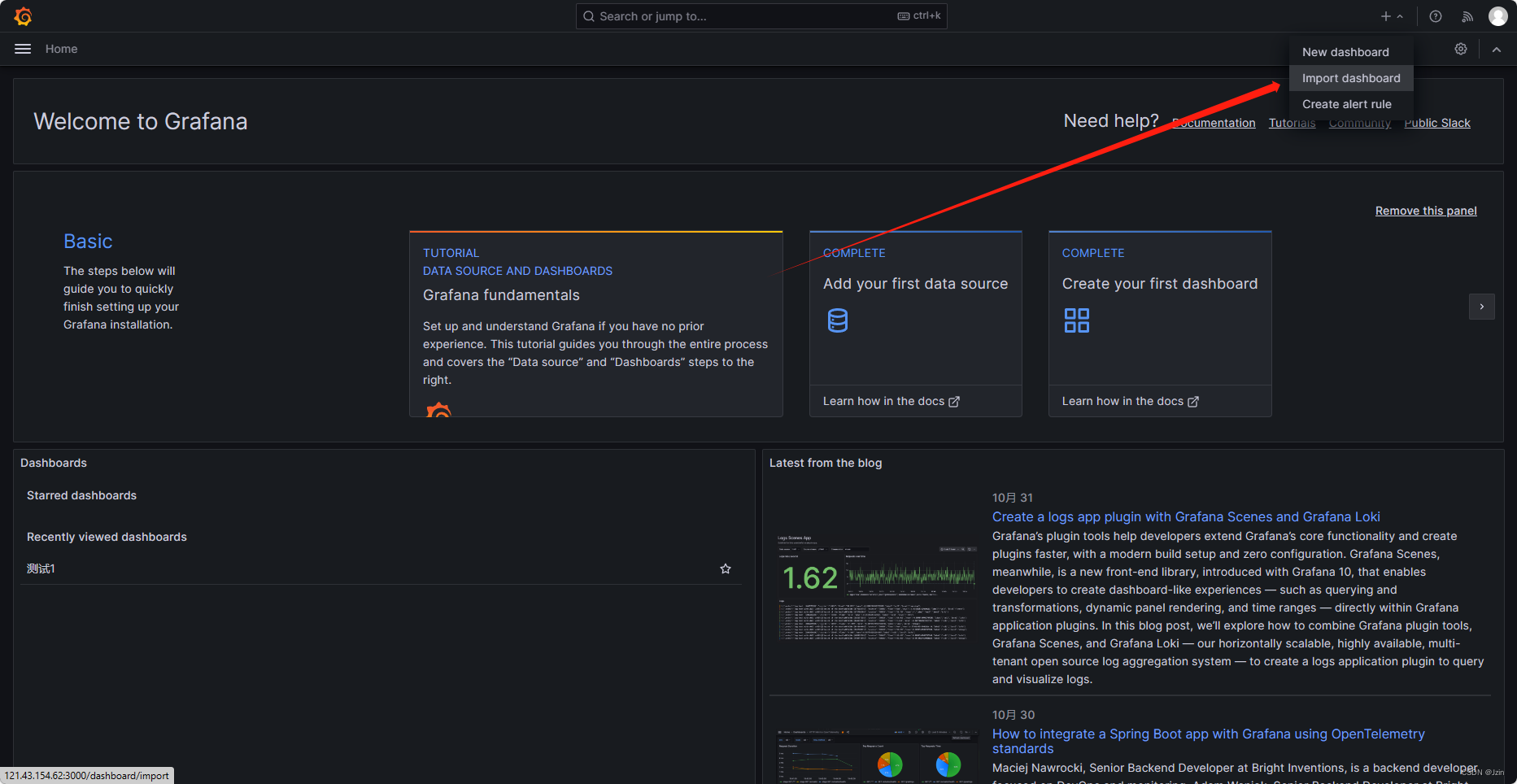
六、导入Grafana模板
官方模板:grafana.com/grafana/dashboards/?search=kafka
比如找一个redis的模板下载:
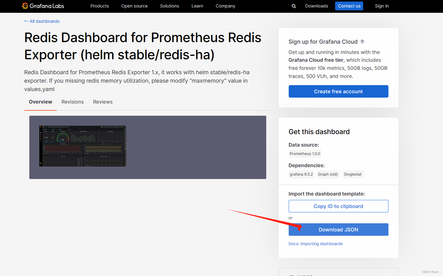
下载完json之后导入到grafana:
可以找其他的模板导入 比如jaeger redis等等
七、guages、counter、histograms指标
guages
最简单的度量指标,只是一个简单的返回值,或者叫瞬时状态,我们想要知道一个队列中的个数
比如:当前的内存使用率、当前的CPU使用率、当前的磁盘使用率、当前的磁盘空间、当前的TCP连接数、当前的流量、当前的QPS、当前的DAU、当前的访问状态、当前的业务接口、当前的产品转换率、当前的充值额度、当前的业务日志、当前的系统日志、当前的网络设备、当前的服务器、当前的机柜、当前的电源、当前的UPS、当前的空调、当前的网络设备、当前的机房环境监控、当前的程序监控
随着时间的推移, 这个值是不断变化的, 这个值有可能增加,有可能减少
Counter
是计数器, 这个值是从0开始累积,在理想状态下,这个值不可能减少
在理想状态下:如果我的服务器重启,同时这个数是放在内存中的
guages和counter是最主要的类型 70%
Histograms
http_res_time 表示http请求的响应时间
nginx
如果我要统计一天的所有访问的平均耗时
如果我们统计下来平均耗时是50ms 但是, 现在中午有一段时间系统卡住了, 1W个请求 平均耗时是在5s,
但是由于我们每天的访问量很大, 1000W访问量,这个5s耗时的请求就被平均掉了
越早发现越好, 有可能是程序的bug,也有可能是系统的bug
50ms以内有多少请求, 50-200ms有多少请求 200ms-500ms有多少请求 500ms-1s有多少请求 1s-5s有多少请求 5s以上有多少请求
分布式图
八、go语言集成prometheus
直接上代码:
package mainimport ("github.com/gin-gonic/gin""github.com/prometheus/client_golang/prometheus""github.com/prometheus/client_golang/prometheus/promauto""github.com/prometheus/client_golang/prometheus/promhttp""time"
)// 声明一个counter
var (opt = promauto.NewCounter(prometheus.CounterOpts{Name: "jzin_test",Help: "just for test",})
)// 每秒自增
func recordMetrics() {for {opt.Inc()time.Sleep(2 * time.Second)}
}// 启动一个http服务,暴露metrics 让prometheus拉取
func main() {go recordMetrics()r := gin.Default()//promauto.NewCounter会把counter注册到defaultRegisterer中 gin.WrapH(promhttp.Handler())会把defaultRegisterer中的metrics暴露出来r.GET("/metrics", gin.WrapH(promhttp.Handler()))_ = r.Run(":8050")
}
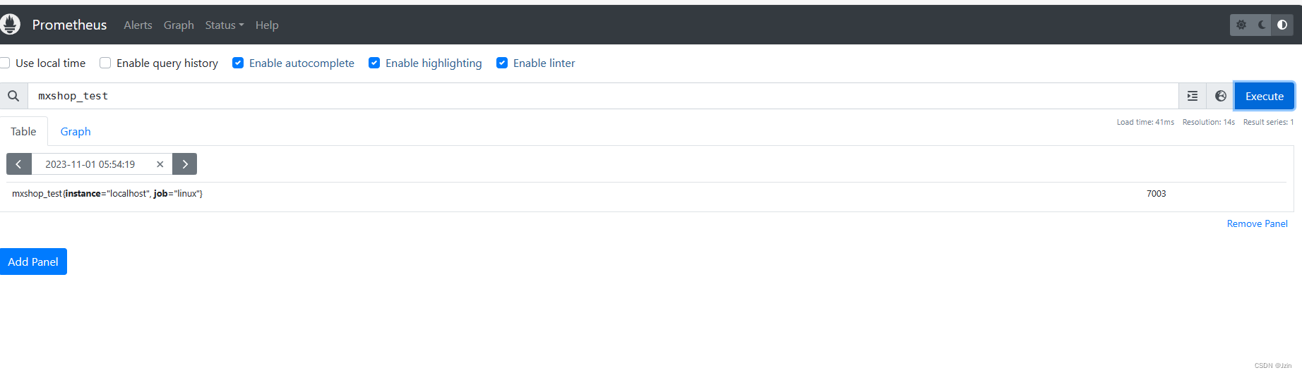
启动后集成到/opt/prometheus里 添加你自己的ip:端口
比如:
global:scrape_interval: 60sevaluation_interval: 60sscrape_configs:- job_name: prometheusstatic_configs:- targets: ['localhost:9090']labels:instance: prometheus- job_name: linuxstatic_configs:- targets: ['172.26.28.143:9100', '你自己的ip:端口']labels:instance: localhost然后重新运行prometheus
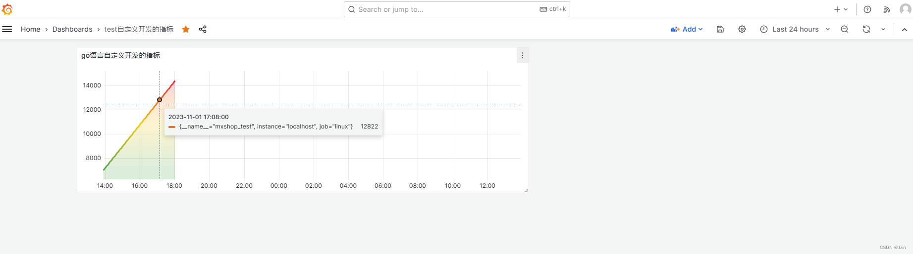
测试:
也可以集成到Garfana中
九、grpc框架集成prometheus
代码有点多 有点复杂 想要的私信吧
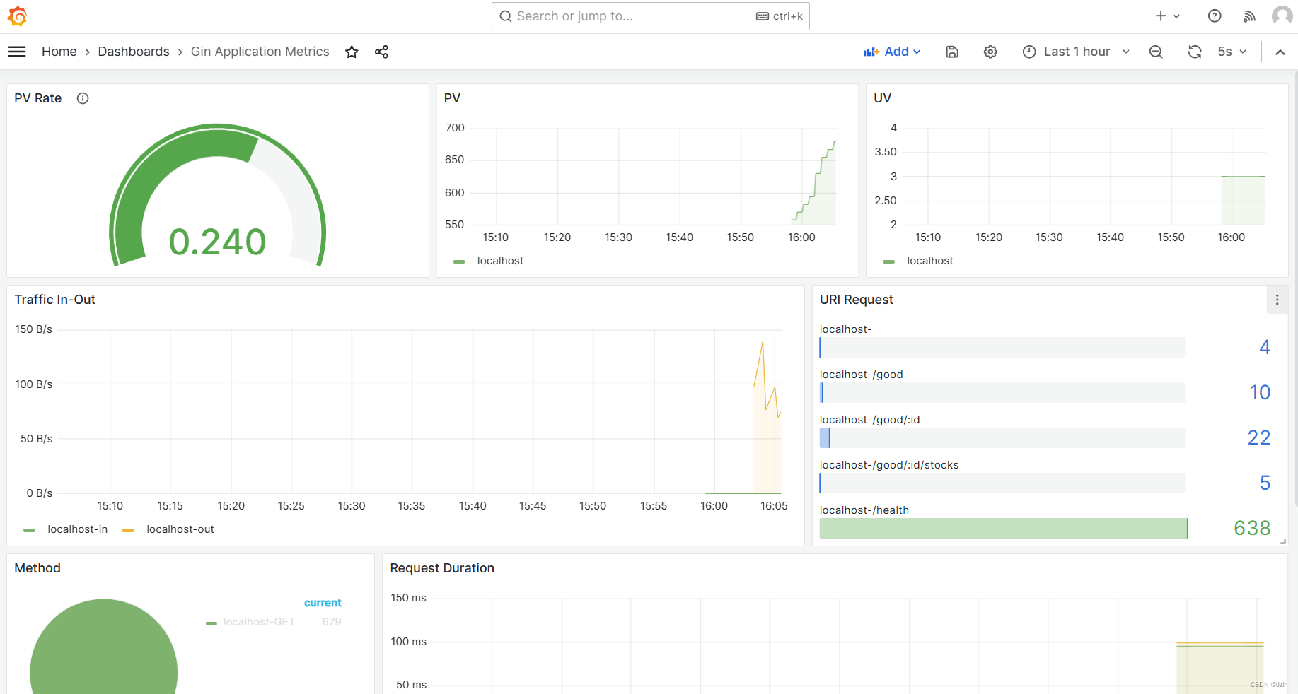
十、gin框架集成prometheus
使用现用的库:https://github.com/penglongli/gin-metrics.git
按照第三方实现即可:
package mainimport ("github.com/gin-gonic/gin""github.com/penglongli/gin-metrics/ginmetrics"
)func main() {r := gin.Default()// get global Monitor objectm := ginmetrics.GetMonitor()// +optional set metric path, default /debug/metricsm.SetMetricPath("/metrics")// +optional set slow time, default 5sm.SetSlowTime(10)// +optional set request duration, default {0.1, 0.3, 1.2, 5, 10}// used to p95, p99m.SetDuration([]float64{0.1, 0.3, 1.2, 5, 10})// set middleware for ginm.Use(r)r.GET("/product/:id", func(ctx *gin.Context) {"productId": ctx.Param("id"),})})_ = r.Run()
}
第三方还提供了garfana的直方图:

看起来效果挺好
json导入:
{"annotations": {"list": [{"builtIn": 1,"datasource": "-- Grafana --","enable": true,"hide": true,"iconColor": "rgba(0, 211, 255, 1)","name": "Annotations & Alerts","type": "dashboard"}]},"editable": true,"gnetId": null,"graphTooltip": 0,"id": 1,"links": [],"panels": [{"datasource": null,"description": "Application request rate every 5 minutes.","fieldConfig": {"defaults": {"custom": {},"mappings": [],"thresholds": {"mode": "absolute","steps": [{"color": "green","value": null},{"color": "red","value": 80}]}},"overrides": []},"gridPos": {"h": 6,"w": 8,"x": 0,"y": 0},"id": 4,"options": {"reduceOptions": {"calcs": ["mean"],"fields": "","values": false},"showThresholdLabels": false,"showThresholdMarkers": true},"pluginVersion": "7.2.0","targets": [{"expr": "rate(gin_request_total[5m])","interval": "","legendFormat": "","refId": "A"}],"timeFrom": null,"timeShift": null,"title": "PV Rate","type": "gauge"},{"aliasColors": {},"bars": false,"dashLength": 10,"dashes": false,"datasource": "Prometheus","description": "","fieldConfig": {"defaults": {"custom": {}},"overrides": []},"fill": 1,"fillGradient": 0,"gridPos": {"h": 6,"w": 8,"x": 8,"y": 0},"hiddenSeries": false,"id": 2,"legend": {"avg": false,"current": false,"max": false,"min": false,"show": true,"total": false,"values": false},"lines": true,"linewidth": 1,"nullPointMode": "null","options": {"alertThreshold": true},"percentage": false,"pluginVersion": "7.2.0","pointradius": 2,"points": false,"renderer": "flot","seriesOverrides": [],"spaceLength": 10,"stack": false,"steppedLine": false,"targets": [{"expr": "gin_request_total","format": "time_series","instant": false,"interval": "","legendFormat": "{{instance}}","refId": "A"}],"thresholds": [],"timeFrom": null,"timeRegions": [],"timeShift": null,"title": "PV","tooltip": {"shared": true,"sort": 0,"value_type": "individual"},"type": "graph","xaxis": {"buckets": null,"mode": "time","name": null,"show": true,"values": []},"yaxes": [{"format": "short","label": null,"logBase": 1,"max": null,"min": null,"show": true},{"format": "short","label": null,"logBase": 1,"max": null,"min": null,"show": true}],"yaxis": {"align": false,"alignLevel": null}},{"aliasColors": {},"bars": false,"dashLength": 10,"dashes": false,"datasource": null,"fieldConfig": {"defaults": {"custom": {}},"overrides": []},"fill": 1,"fillGradient": 0,"gridPos": {"h": 6,"w": 8,"x": 16,"y": 0},"hiddenSeries": false,"id": 6,"legend": {"avg": false,"current": false,"max": false,"min": false,"show": true,"total": false,"values": false},"lines": true,"linewidth": 1,"nullPointMode": "null","options": {"alertThreshold": true},"percentage": false,"pluginVersion": "7.2.0","pointradius": 2,"points": false,"renderer": "flot","seriesOverrides": [],"spaceLength": 10,"stack": false,"steppedLine": false,"targets": [{"expr": "gin_request_uv_total","interval": "","legendFormat": "{{instance}}","refId": "A"}],"thresholds": [],"timeFrom": null,"timeRegions": [],"timeShift": null,"title": "UV","tooltip": {"shared": true,"sort": 0,"value_type": "individual"},"type": "graph","xaxis": {"buckets": null,"mode": "time","name": null,"show": true,"values": []},"yaxes": [{"format": "short","label": null,"logBase": 1,"max": null,"min": null,"show": true},{"format": "short","label": null,"logBase": 1,"max": null,"min": null,"show": true}],"yaxis": {"align": false,"alignLevel": null}},{"aliasColors": {},"bars": false,"dashLength": 10,"dashes": false,"datasource": null,"fieldConfig": {"defaults": {"custom": {},"unit": "Bps"},"overrides": []},"fill": 1,"fillGradient": 0,"gridPos": {"h": 8,"w": 15,"x": 0,"y": 6},"hiddenSeries": false,"id": 12,"legend": {"avg": false,"current": false,"max": false,"min": false,"show": true,"total": false,"values": false},"lines": true,"linewidth": 1,"nullPointMode": "null","options": {"alertThreshold": true},"percentage": false,"pluginVersion": "7.2.0","pointradius": 2,"points": false,"renderer": "flot","seriesOverrides": [],"spaceLength": 10,"stack": false,"steppedLine": false,"targets": [{"expr": "rate(gin_request_body_total[5m])","interval": "","legendFormat": "{{instance}}-in","refId": "A"},{"expr": "rate(gin_response_body_total[5m])","interval": "","legendFormat": "{{instance}}-out","refId": "B"}],"thresholds": [],"timeFrom": null,"timeRegions": [],"timeShift": null,"title": "Traffic In-Out","tooltip": {"shared": true,"sort": 0,"value_type": "individual"},"type": "graph","xaxis": {"buckets": null,"mode": "time","name": null,"show": true,"values": []},"yaxes": [{"format": "Bps","label": null,"logBase": 1,"max": null,"min": null,"show": true},{"format": "bytes","label": null,"logBase": 1,"max": null,"min": null,"show": true}],"yaxis": {"align": false,"alignLevel": null}},{"cacheTimeout": null,"datasource": null,"fieldConfig": {"defaults": {"custom": {"align": null,"filterable": false},"mappings": [],"thresholds": {"mode": "absolute","steps": [{"color": "blue","value": null},{"color": "green","value": 80}]},"unit": "none"},"overrides": []},"gridPos": {"h": 8,"w": 9,"x": 15,"y": 6},"id": 10,"interval": null,"links": [],"options": {"displayMode": "basic","orientation": "horizontal","reduceOptions": {"calcs": ["last"],"fields": "","values": false},"showUnfilled": true},"pluginVersion": "7.2.0","targets": [{"expr": "sum by(uri, instance) (gin_uri_request_total)","format": "time_series","instant": false,"interval": "","intervalFactor": 1,"legendFormat": "{{instance}}-{{uri}}","refId": "A"}],"timeFrom": null,"timeShift": null,"title": "URI Request","type": "bargauge"},{"aliasColors": {},"breakPoint": "50%","cacheTimeout": null,"combine": {"label": "Others","threshold": 0},"datasource": null,"decimals": null,"fieldConfig": {"defaults": {"custom": {"align": null,"filterable": false},"mappings": [],"thresholds": {"mode": "absolute","steps": [{"color": "blue","value": null},{"color": "green","value": 80}]},"unit": "none"},"overrides": []},"fontSize": "80%","format": "none","gridPos": {"h": 7,"w": 7,"x": 0,"y": 14},"id": 13,"interval": null,"legend": {"show": true,"values": true},"legendType": "Right side","links": [],"nullPointMode": "connected","pieType": "pie","pluginVersion": "7.2.0","strokeWidth": 1,"targets": [{"expr": "sum by(method, instance) (gin_uri_request_total)","format": "time_series","instant": false,"interval": "","intervalFactor": 1,"legendFormat": "{{instance}}-{{method}}","refId": "A"}],"timeFrom": null,"timeShift": null,"title": "Method","type": "grafana-piechart-panel","valueName": "current"},{"aliasColors": {},"bars": false,"dashLength": 10,"dashes": false,"datasource": null,"fieldConfig": {"defaults": {"custom": {},"unit": "s"},"overrides": []},"fill": 1,"fillGradient": 0,"gridPos": {"h": 7,"w": 17,"x": 7,"y": 14},"hiddenSeries": false,"id": 16,"legend": {"avg": false,"current": false,"max": false,"min": false,"show": true,"total": false,"values": false},"lines": true,"linewidth": 1,"nullPointMode": "null","options": {"alertThreshold": true},"percentage": false,"pluginVersion": "7.2.0","pointradius": 2,"points": false,"renderer": "flot","seriesOverrides": [],"spaceLength": 10,"stack": false,"steppedLine": false,"targets": [{"expr": "histogram_quantile(0.95, sum (rate(gin_request_duration_bucket[5m])) by (le, instance))","interval": "","legendFormat": "p95","refId": "A"},{"expr": "histogram_quantile(0.99, sum (rate(gin_request_duration_bucket[5m])) by (le, instance))","interval": "","legendFormat": "p99","refId": "B"},{"expr": "sum (gin_request_duration_sum) / sum(gin_request_duration_count)","interval": "","legendFormat": "avg","refId": "C"}],"thresholds": [],"timeFrom": null,"timeRegions": [],"timeShift": null,"title": "Request Duration","tooltip": {"shared": true,"sort": 0,"value_type": "individual"},"type": "graph","xaxis": {"buckets": null,"mode": "time","name": null,"show": true,"values": []},"yaxes": [{"format": "s","label": null,"logBase": 1,"max": null,"min": null,"show": true},{"format": "bytes","label": null,"logBase": 1,"max": null,"min": null,"show": true}],"yaxis": {"align": false,"alignLevel": null}},{"aliasColors": {},"breakPoint": "50%","cacheTimeout": null,"combine": {"label": "Others","threshold": 0},"datasource": null,"decimals": null,"description": "","fieldConfig": {"defaults": {"custom": {"align": null,"filterable": false},"mappings": [],"thresholds": {"mode": "absolute","steps": [{"color": "blue","value": null},{"color": "green","value": 80}]},"unit": "none"},"overrides": []},"fontSize": "80%","format": "none","gridPos": {"h": 5,"w": 7,"x": 0,"y": 21},"id": 14,"interval": null,"legend": {"show": true,"values": true},"legendType": "Right side","links": [],"nullPointMode": "connected","pieType": "pie","pluginVersion": "7.2.0","strokeWidth": 1,"targets": [{"expr": "sum by(code, instance) (gin_uri_request_total)","format": "time_series","instant": false,"interval": "","intervalFactor": 1,"legendFormat": "{{instance}}-{{code}}","refId": "A"}],"timeFrom": null,"timeShift": null,"title": "Code","type": "grafana-piechart-panel","valueName": "current"},{"cacheTimeout": null,"datasource": null,"fieldConfig": {"defaults": {"custom": {"align": null,"filterable": false},"mappings": [],"thresholds": {"mode": "absolute","steps": [{"color": "blue","value": null},{"color": "green","value": 80}]},"unit": "none"},"overrides": []},"gridPos": {"h": 5,"w": 17,"x": 7,"y": 21},"id": 19,"interval": null,"links": [],"options": {"displayMode": "basic","orientation": "horizontal","reduceOptions": {"calcs": ["last"],"fields": "","values": false},"showUnfilled": true},"pluginVersion": "7.2.0","targets": [{"expr": "sum by(uri, instance) (gin_slow_request_total)","format": "time_series","instant": false,"interval": "","intervalFactor": 1,"legendFormat": "{{instance}}-{{uri}}","refId": "A"}],"timeFrom": null,"timeShift": null,"title": "Slow Request(default 5s)","type": "bargauge"}],"refresh": "5s","schemaVersion": 26,"style": "dark","tags": [],"templating": {"list": []},"time": {"from": "now-1h","to": "now"},"timepicker": {},"timezone": "","title": "Gin Application Metrics","uid": "FDB061FMz","version": 11
}
如果直方图报错Panel plugin not found: grafana-piechart-panel
那就给garfana安装插件
下载安装后放到插件目录/var/lib/grafana/plugins后重启grafana就可以了。
wget  https://grafana.com/api/plugins/grafana-piechart-panel/versions/latest/download -O grafana-piechart-panel.zip
unzip grafana-piechart-panel.zip
mv grafana-piechart-panel grafana_data/plugins/
chown -R 472:472 *
docker restart grafana
把程序放到自己的服务器中 多写几条get post命令进行测试:
测试结果:
相关文章:
【监控指标】监控系统-prometheus、grafana。容器化部署。go语言 gin框架、gRPC框架的集成
文章目录 一、监控有哪些指标二、prometheus、grafana架构Prometheus 组件Grafana 组件架构优点 三、安装prometheus和node-exporter1. docker pull镜像2. 启动node-exporter3. 启动prometheus 四、promql基本语法五、grafana的安装和使用1. 新建空文件夹grafana-storage&#…...

时序分解 | Matlab实现PSO-VMD粒子群算法优化变分模态分解时间序列信号分解
时序分解 | Matlab实现PSO-VMD粒子群算法优化变分模态分解时间序列信号分解 目录 时序分解 | Matlab实现PSO-VMD粒子群算法优化变分模态分解时间序列信号分解效果一览基本介绍程序设计参考资料 效果一览 基本介绍 PSO-VMD粒子群算法PSO优化VMD变分模态分解 可直接运行 分解效果…...
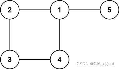
leetcode 684. 冗余连接
树可以看成是一个连通且 无环 的 无向 图。 给定往一棵 n 个节点 (节点值 1~n) 的树中添加一条边后的图。添加的边的两个顶点包含在 1 到 n 中间,且这条附加的边不属于树中已存在的边。图的信息记录于长度为 n 的二维数组 edges ,edges[i] …...
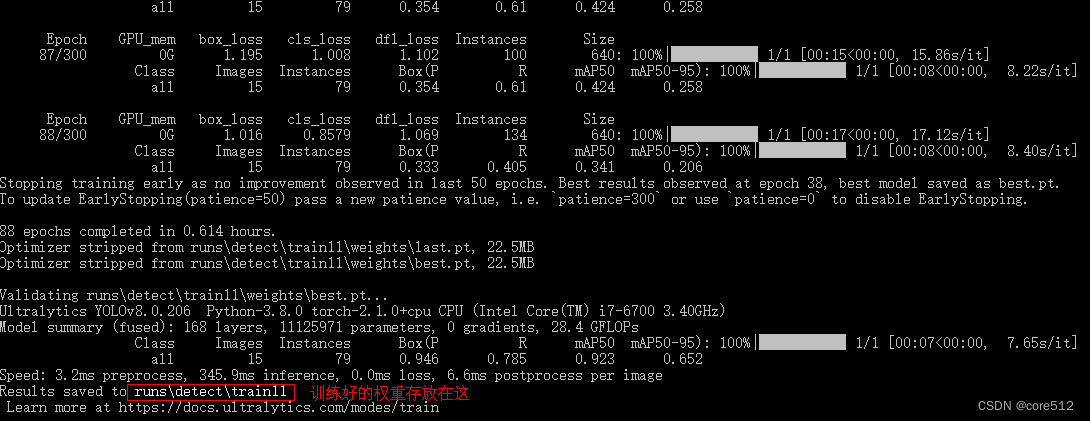
yolov8模型训练、目标跟踪
一、准备条件 1.下载yolov8 https://github.com/ultralytics/ultralytics2.安装python https://www.python.org/ftp/python/3.8.0/python-3.8.0-amd64.exe3.安装依赖 进入ultralytics-main,执行: pip install -r requirements.txt pip install -U ul…...
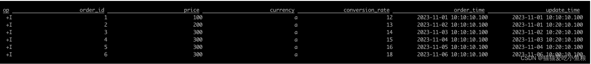
Flink SQL Regular Join 、Interval Join、Temporal Join、Lookup Join 详解
Flink ⽀持⾮常多的数据 Join ⽅式,主要包括以下三种: 动态表(流)与动态表(流)的 Join动态表(流)与外部维表(⽐如 Redis)的 Join动态表字段的列转⾏…...

如何在搜索引擎中应用AI大语言模型,提高企业生产力?
人工智能尤其是大型语言模型的应用,重塑了我们与信息交互的方式,也为企业带来了重大的变革。将基于大模型的检索增强生成(RAG)集成到业务实践中,不仅是一种趋势,更是一种必要。它有助于实现数据驱动型决策&…...

实验七 组合器模式的应用
实验目的 1)掌握组合器模式(composite)的特点 2 分析具体问题,使用组合器模式进行设计。 实验内容和要求 在例3.3的设计中,添加一个空军大队( Wing)类,该类与Squadron、Group类是平行的,因此应该继承了AirU…...

Springboot实现人脸识别与WebSocket长连接的实现
0.什么是WebSocket,由于普通的请求是间断式发送的,如果要同一时间发生大量的请求,必然导致响应速度慢(因为根据tcp协议要经过三层握手,如果不持续发送,就会导致n多次握手,关闭连接,打开连接) 1.业务需求: 由于我需要使用java来处理视频的问题,视频其实就是图片,相当于每张图片…...
智能安全帽功能-EIS智能防抖摄像头4G定位视频语音气体检测
智能安全帽是一种集成多种智能功能的产品,例如实时定位、语音对讲、健康监测和AI智能预警等。这些丰富的功能能够更好地帮助工人开展工作,并提升安全保障水平。智能安全帽在各个行业中的应用越来越广泛。尤其在工程建设领域,项目管理和工作安…...

TEMU跨境平台珠宝首饰RSL报告如何办理?
首饰或者产品TEMU拼多多跨境平台要求的RSL报告如何办理? 珠宝首饰上架前必须进行RSL Report(欧盟禁限用化学物质检测报告) 随着人们对珠宝首饰的要求越来越高,为了确保珠宝首饰的安全性,欧盟REACH法规规定,…...

51单片机的篮球计分器液晶LCD1602显示( proteus仿真+程序+原理图+PCB+设计报告+讲解视频)
51单片机的篮球计分器液晶LCD1602显示 📑1.主要功能:📑讲解视频:📑2.仿真📑3. 程序代码📑4. 原理图📑5. PCB图📑6. 设计报告📑7. 设计资料内容清单&&…...
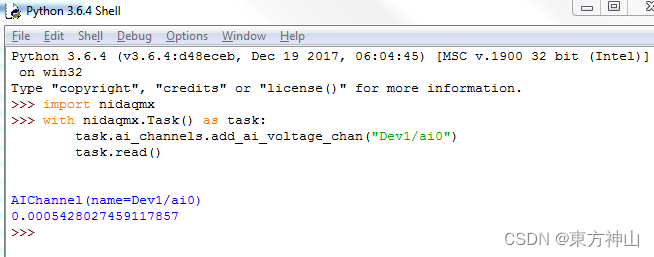
【NI-DAQmx入门】NI-DAQmx之Python
NI-DAQmx Python GitHub资源: NI-DAQmx Python 文档说明:NI-DAQmx Python Documentation — NI-DAQmx Python API 0.9 documentation nidaqmx支持 CPython 3.7和 PyPy3,需要注意的是多支持USB DAQ和PCI DAQ,cDAQ需要指定…...

YoloV8目标检测与实例分割——目标检测onnx模型推理
一、模型转换 1.onnxruntime ONNX Runtime(ONNX Runtime或ORT)是一个开源的高性能推理引擎,用于部署和运行机器学习模型。它的设计目标是优化执行使用Open Neural Network Exchange(ONNX)格式定义的模型,…...
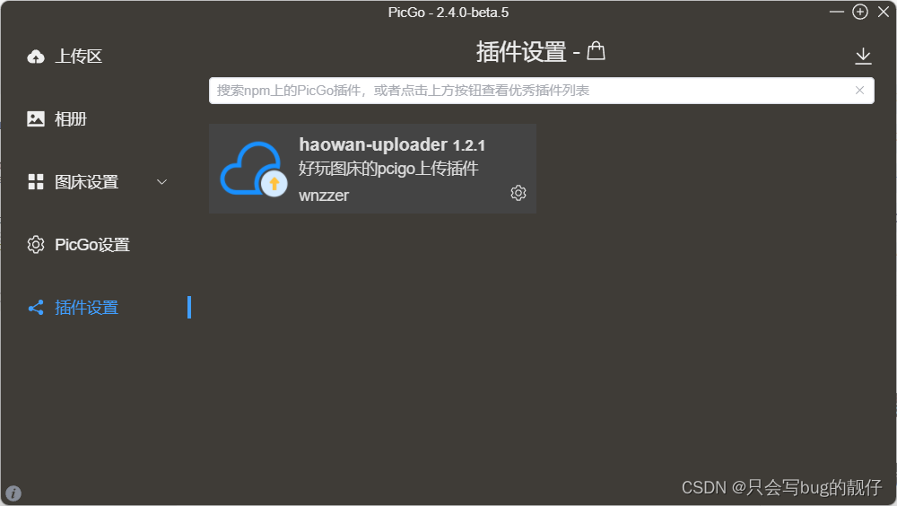
pcigo图床插件的简单开发
1.前言: 如果想写一个图床并且投入使用,那么,接入picgo一定是一个不错的选择。picgo有着windows,mac,linux等多个客户端版本。实用且方便。 2. 开发的准备: 2.0. 需要安装一个node node这里我就不详细说…...

Find My手机保护壳|苹果Find My与手机保护壳结合,智能防丢,全球定位
随着科技水平的快速发展,科技美容这一行业做为新型产业新生而出。时尚IT品牌随着市场的多元化发展。针对手机品牌和功能的增加而呈多样化,将手机保护壳按质地分有PC壳,皮革 ,硅胶,布料,硬塑,皮套…...

encode和decode的区别
字节序列和字符串是Python中两种不同的数据类型,它们的主要区别在于表示和处理方式! 字节序列(Bytes): 字节序列是一种二进制数据类型,它由一系列字节组成。字节是计算机存储信息的基本单位,每…...

建设项目管理中的 5 大预算挑战
为建设项目管理制定可靠、准确的预算是一项艰巨的任务,对于中小型建筑企业来说尤其如此。预算必须精确,同时还要考虑到每项工作的独特性和复杂性。 一项建筑行业相关调查统计了参与施工预算流程的人员所面临的最大挑战,分别是时间、预算、不…...

vue2 集成 - 超图-SuperMap iClient3D for WebGL
1:下载SuperMap iClient3D for WebGL SuperMap iClient3D for WebGL产品包 打开资源目录如下 2:格式化项目中所用的依赖包 开发指南 从超图官网下载SuperMap iClient3D 11i (2023) SP1 for WebGL_CN.zip解压后,将Build目录下的SuperMap3D复制到项目中 \public\static…...

FPGA设计过程中有关数据之间的并串转化
1.原理 并串转化是指的是完成串行传输和并行传输两种传输方式之间的转换的技术,通过移位寄存器可以实现串并转换。 串转并,将数据移位保存在寄存器中,再将寄存器的数值同时输出; 并转串,将数据先进行移位࿰…...

hologres基础知识一文全
1 功能特性 1.1多场景查询分析 Hologres支持行存、列存、行列共存等多种存储模式和索引类型,同时满足简单查询、复杂查询、即席查询等多样化的分析查询需求。Hologres使用大规模并行处理架构,分布式处理SQL,提高资源利用率,实现海量数据极速分析。 亚秒级交互式分析 Holo…...
)
归并排序实战:如何用分治思想高效计算逆序对(附Python代码)
归并排序实战:如何用分治思想高效计算逆序对(附Python代码) 在金融风控系统中,我们常需要评估交易数据的异常波动;在推荐算法里,用户行为序列的混乱程度直接影响推荐效果。这些场景背后都藏着一个关键指标—…...

Fish-Speech-1.5在虚拟偶像中的应用:个性化语音合成方案
Fish-Speech-1.5在虚拟偶像中的应用:个性化语音合成方案 1. 引言 虚拟偶像正在改变数字娱乐的格局,但要让这些数字角色真正"活起来",声音的表现力至关重要。传统的语音合成技术往往显得生硬机械,缺乏真实感和情感共鸣…...

ssm+java2026年毕设生产安全法执法依据库管理【源码+论文】
本系统(程序源码)带文档lw万字以上 文末可获取一份本项目的java源码和数据库参考。系统程序文件列表开题报告内容一、选题背景关于法律信息管理与事故处理系统的研究,现有研究主要以通用性的信息管理系统和简单的法律咨询平台为主,…...

华为eNSP进阶实战:从零构建企业级网络,打通仿真与认证的最后一公里
1. 为什么你需要掌握华为eNSP? 作为一名网络工程师,或者正在备考华为HCIP/HCIE认证的学习者,你一定遇到过这样的困扰:想要搭建一个完整的企业级网络环境进行实验,但硬件设备成本高昂,物理环境搭建复杂。这时…...

跌破1500元的荣耀性价比神机,除CPU略差,其它方面都超值!
荣耀云空间 "荣耀X70虽涨价300元,但PDD百亿补贴后仅1464元,旗舰外观8300mAh电池顶级防护6年流畅系统,1500元档性价比之王,现在不买更待何时?" 继OV之后,第三家悄悄调价的厂商已经被爆出了&…...

Langchain架构解析:从文本到向量再到答案的完整流程详解
Langchain架构解析:从文本到向量再到答案的完整流程详解 当你第一次听说Langchain时,可能会被那些专业术语和复杂流程搞得一头雾水。别担心,今天我们就用最接地气的方式,把这个看似高深的技术拆解成容易理解的模块。Langchain本质…...

【JavaSE】JavaSE入门--探索Java的核心特性与应用场景
1. JavaSE入门:为什么选择Java? 第一次接触Java时,我被它"一次编写,到处运行"的特性深深吸引。记得2013年做毕业设计时,我需要在Windows上开发一个能在Linux服务器运行的程序,正是Java帮我解决了…...

Granite TimeSeries FlowState R1模型效果深度评测:对比传统统计方法与深度学习模型
Granite TimeSeries FlowState R1模型效果深度评测:对比传统统计方法与深度学习模型 时序预测这事儿,就像给未来的天气画一张草图,谁都想画得更准一点。过去,我们手里有像ARIMA、Prophet这样的经典“画笔”,后来深度学…...

Artifactory-oos私有Maven仓库:从零搭建到企业级组件托管实战
1. 为什么企业需要私有Maven仓库 记得去年我们团队接手一个大型金融项目时,遇到了一个典型问题:十几个模块都在重复使用相同的支付SDK,每次版本更新都要手动替换所有项目的jar包。更糟的是,某个同事不小心用了旧版本导致线上事故。…...

从视频到空间:面向智慧军营的三维作战感知与认知决策平台
《从视频到空间:面向智慧军营的三维作战感知与认知决策平台》副标题:基于 Pixel-to-Space 的空间认知引擎与战术智能体系发布单位:镜像视界(浙江)科技有限公司一、执行摘要随着信息化战争向智能化战争演进,…...