BikeDNA(九) 特征匹配
BikeDNA(九) 特征匹配
特征匹配采用参考数据并尝试识别 OSM 数据集中的相应特征。 特征匹配是比较单个特征而不是研究区域网格单元水平上的特征特征的必要前提。
方法
将两个道路数据集中的特征与其数字化特征的方式以及边缘之间潜在的一对多关系进行匹配(例如,一个数据集仅映射道路中心线,而另一个数据集映射每辆自行车的几何形状) 车道)并不是一项简单的任务。
这里使用的方法将所有网络边缘转换为统一长度的较小段,然后再寻找参考和 OSM 数据之间的潜在匹配。 匹配是根据对象之间的缓冲距离、角度和无向 Hausdorff 距离完成的,并且基于 Koukoletsos et al. (2012) and Will (2014)。
根据匹配结果,计算以下值:
- 匹配和不匹配边缘的总数和每个网格单元的数量和长度
- 匹配边缘的属性比较:它们对自行车基础设施受保护或不受保护的分类是否相同?
解释
直观地探索特征匹配结果非常重要,因为匹配的成功率会影响如何解释匹配数的分析。
如果两个数据集中的特征被不同地数字化 - 例如 如果一个数据集将自行车轨道数字化为大部分直线,而另一个数据集包含更多蜿蜒轨道,则匹配将失败。 如果它们彼此放置得太远,也会出现这种情况。 如果可以通过视觉确认两个数据集中确实存在相同的特征,则缺乏匹配表明两个数据集中的几何形状差异太大。 然而,如果可以确认大多数真实的相应特征已被识别,则区域中缺乏匹配表明存在错误或遗漏。
特征匹配的计算成本很高,并且需要一段时间才能计算。 对于此存储库中提供的测试数据(具有大约 800 公里的 OSM 网络),单元运行大约需要 20 分钟。
# Load libraries, settings and dataimport json
import numbers
import os.path
import pickleimport contextily as cx
import folium
import geopandas as gpd
import matplotlib.colors as colors
import matplotlib.pyplot as plt
import osmnx as ox
import pandas as pd
import yaml
import numpy as npfrom src import evaluation_functions as eval_func
from src import matching_functions as match_func
from src import plotting_functions as plot_func# Read in dictionaries with settings
%run ../settings/yaml_variables.py
%run ../settings/plotting.py
%run ../settings/tiledict.py
%run ../settings/paths.py# # Load data
%run ../settings/load_osmdata.py
%run ../settings/load_refdata.py
%run ../settings/df_styler.py# Combine grid geodataframes
grid = osm_grid.merge(ref_grid)
assert len(grid) == len(osm_grid) == len(ref_grid)
D:\tmp_resource\BikeDNA-main\BikeDNA-main\scripts\settings\plotting.py:49: MatplotlibDeprecationWarning: The get_cmap function was deprecated in Matplotlib 3.7 and will be removed two minor releases later. Use ``matplotlib.colormaps[name]`` or ``matplotlib.colormaps.get_cmap(obj)`` instead.cmap = cm.get_cmap(cmap_name, n)
D:\tmp_resource\BikeDNA-main\BikeDNA-main\scripts\settings\plotting.py:46: MatplotlibDeprecationWarning: The get_cmap function was deprecated in Matplotlib 3.7 and will be removed two minor releases later. Use ``matplotlib.colormaps[name]`` or ``matplotlib.colormaps.get_cmap(obj)`` instead.cmap = cm.get_cmap(cmap_name)OSM graphs loaded successfully!
OSM data loaded successfully!
Reference graphs loaded successfully!
Reference data loaded successfully!<string>:49: MatplotlibDeprecationWarning: The get_cmap function was deprecated in Matplotlib 3.7 and will be removed two minor releases later. Use ``matplotlib.colormaps[name]`` or ``matplotlib.colormaps.get_cmap(obj)`` instead.
<string>:46: MatplotlibDeprecationWarning: The get_cmap function was deprecated in Matplotlib 3.7 and will be removed two minor releases later. Use ``matplotlib.colormaps[name]`` or ``matplotlib.colormaps.get_cmap(obj)`` instead.
1. 匹配特征
1.1 运行并绘制特征匹配
在特征匹配中,用户必须指出:
- 线段长度(所有要素在匹配之前分割成的线段长度,以米为单位)(segment_length)。
- 用于查找潜在匹配项的缓冲区距离(即可以表示同一对象的两个段之间的最大距离)(buffer_dist)。
- 可以被视为匹配的要素之间的最大豪斯多夫距离(在本文中,它指的是两个几何图形之间的最大距离。例如,长度为 25 米的线段 A 可能位于线段 10 米的缓冲距离内 B,但如果它们相互垂直,Hausdorff 距离将大于 10 米)(hausdorff_threshold)。
- 线段之间的角度阈值,然后它们不再被视为潜在匹配(angular_threshold)。
# Define feature matching user settingssegment_length = 10  # The shorter the segments, the longer the matching process will take. For cities with a gridded street network with streets as straight lines, longer segments will usually work fine
buffer_dist = 15
hausdorff_threshold = 17
angular_threshold = 30for s in [segment_length, buffer_dist, hausdorff_threshold, angular_threshold]:assert isinstance(s, int) or isinstance(s, float), print("Settings must be integer or float values!")
osm_seg_fp = compare_results_data_fp + f"osm_segments_{segment_length}.gpkg"
ref_seg_fp = compare_results_data_fp + f"ref_segments_{segment_length}.gpkg"if os.path.exists(osm_seg_fp) and os.path.exists(ref_seg_fp):osm_segments = gpd.read_file(osm_seg_fp)ref_segments = gpd.read_file(ref_seg_fp)print("Segments have already been created! Continuing with existing segment data.")print("\n")else:print("Creating edge segments for OSM and reference data...")osm_segments = match_func.create_segment_gdf(osm_edges_simplified, segment_length=segment_length)osm_segments.rename(columns={"osmid": "org_osmid"}, inplace=True)osm_segments["osmid"] = osm_segments["edge_id"]  # Because matching function assumes an id column names osmid as unique id for edgesosm_segments.set_crs(study_crs, inplace=True)osm_segments.dropna(subset=["geometry"], inplace=True)ref_segments = match_func.create_segment_gdf(ref_edges_simplified, segment_length=segment_length)ref_segments.set_crs(study_crs, inplace=True)ref_segments.rename(columns={"seg_id": "seg_id_ref"}, inplace=True)ref_segments.dropna(subset=["geometry"], inplace=True)print("Segments created successfully!")print("\n")osm_segments.to_file(osm_seg_fp)ref_segments.to_file(ref_seg_fp)print("Segments saved!")
Creating edge segments for OSM and reference data...d:\work\miniconda3\envs\bikeDNA\Lib\site-packages\geopandas\geoseries.py:645: FutureWarning: the convert_dtype parameter is deprecated and will be removed in a future version.  Do ``ser.astype(object).apply()`` instead if you want ``convert_dtype=False``.result = super().apply(func, convert_dtype=convert_dtype, args=args, **kwargs)
d:\work\miniconda3\envs\bikeDNA\Lib\site-packages\geopandas\geoseries.py:645: FutureWarning: the convert_dtype parameter is deprecated and will be removed in a future version.  Do ``ser.astype(object).apply()`` instead if you want ``convert_dtype=False``.result = super().apply(func, convert_dtype=convert_dtype, args=args, **kwargs)
d:\work\miniconda3\envs\bikeDNA\Lib\site-packages\geopandas\geoseries.py:645: FutureWarning: the convert_dtype parameter is deprecated and will be removed in a future version.  Do ``ser.astype(object).apply()`` instead if you want ``convert_dtype=False``.result = super().apply(func, convert_dtype=convert_dtype, args=args, **kwargs)
d:\work\miniconda3\envs\bikeDNA\Lib\site-packages\geopandas\geoseries.py:645: FutureWarning: the convert_dtype parameter is deprecated and will be removed in a future version.  Do ``ser.astype(object).apply()`` instead if you want ``convert_dtype=False``.result = super().apply(func, convert_dtype=convert_dtype, args=args, **kwargs)Segments created successfully!Segments saved!
matches_fp = f"../../results/compare/{study_area}/data/segment_matches_{buffer_dist}_{hausdorff_threshold}_{angular_threshold}.pickle"if os.path.exists(matches_fp):with open(matches_fp, "rb") as fp:segment_matches = pickle.load(fp)print(f"Segment matching has already been performed. Loading existing segment matches, matched with a buffer distance of {buffer_dist} meters, a Hausdorff distance of {hausdorff_threshold} meters, and a max angle of {angular_threshold} degrees.")print("\n")else:print(f"Starting matching process using a buffer distance of {buffer_dist} meters, a Hausdorff distance of {hausdorff_threshold} meters, and a max angle of {angular_threshold} degrees.")print("\n")buffer_matches = match_func.overlay_buffer(reference_data=ref_segments,osm_data=osm_segments,ref_id_col="seg_id_ref",osm_id_col="seg_id",dist=buffer_dist,)print("Buffer matches found! Continuing with final matching process...")print("\n")segment_matches = match_func.find_matches_from_buffer(buffer_matches=buffer_matches,osm_edges=osm_segments,reference_data=ref_segments,angular_threshold=angular_threshold,hausdorff_threshold=hausdorff_threshold,)print("Feature matching completed!")with open(matches_fp, "wb") as f:pickle.dump(segment_matches, f)
Starting matching process using a buffer distance of 15 meters, a Hausdorff distance of 17 meters, and a max angle of 30 degrees.Buffer matches found! Continuing with final matching process...60946 reference segments were matched to OSM edges
2749 reference segments were not matched
Feature matching completed!
osm_matched_segments = osm_segments.loc[osm_segments.seg_id.isin(segment_matches.matches_id)]
osm_unmatched_segments = osm_segments.loc[~osm_segments.seg_id.isin(segment_matches.matches_id)]
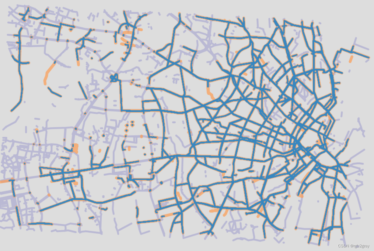
# Interactive plot of segment matchesosm_edges_simplified_folium = plot_func.make_edgefeaturegroup(gdf=osm_edges_simplified,mycolor=pdict["osm_seg"],myweight=pdict["osm_weight"],nametag="OSM: all edges",show_edges=True,myalpha=pdict["osm_alpha"],
)ref_edges_simplified_folium = plot_func.make_edgefeaturegroup(gdf=ref_edges_simplified,mycolor=pdict["ref_seg"],myweight=pdict["ref_weight"],nametag=f"{reference_name}: all edges",show_edges=True,myalpha=pdict["ref_alpha"],
)segment_matches_folium = plot_func.make_edgefeaturegroup(gdf=segment_matches,mycolor=pdict["mat_seg"],myweight=pdict["mat_weight"],nametag=f"OSM and {reference_name}: matched segments",show_edges=True,myalpha=pdict["mat_alpha"],
)m = plot_func.make_foliumplot(feature_groups=[osm_edges_simplified_folium,ref_edges_simplified_folium,segment_matches_folium,],layers_dict=folium_layers,center_gdf=osm_nodes_simplified,center_crs=osm_nodes_simplified.crs,
)bounds = plot_func.compute_folium_bounds(osm_nodes_simplified)
m.fit_bounds(bounds)m.save(compare_results_inter_maps_fp+ f"segment_matches_{buffer_dist}_{hausdorff_threshold}_{angular_threshold}_compare.html"
)display(m)
print("Interactive map saved at " + compare_results_inter_maps_fp.lstrip("../")+ f"segment_matches_{buffer_dist}_{hausdorff_threshold}_{angular_threshold}_compare.html")
Interactive map saved at results/COMPARE/cph_geodk/maps_interactive/segment_matches_15_17_30_compare.html
# Plot matched and unmatched featuresset_renderer(renderer_map)# OSM
fig, ax = plt.subplots(1, 1, figsize=pdict["fsmap"])osm_matched_segments.plot(ax=ax, color=pdict["match"], label="matched"
)osm_unmatched_segments.plot(ax=ax, color=pdict["nomatch"], label="unmatched"
)cx.add_basemap(ax=ax, crs=study_crs, source=cx_tile_2)
ax.set_title(area_name + ": OSM matched & unmatched features")
ax.set_axis_off()
ax.legend()plot_func.save_fig(fig, compare_results_static_maps_fp + f"matched_OSM_{buffer_dist}_{hausdorff_threshold}_{angular_threshold}_compare")# REF
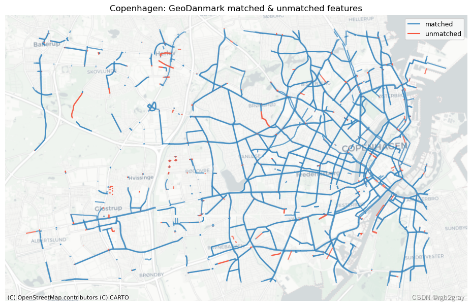
ref_matched_segments = segment_matches
ref_unmatched_segments = ref_segments.loc[~ref_segments.seg_id_ref.isin(segment_matches.seg_id_ref)]fig, ax = plt.subplots(1, 1, figsize=pdict["fsmap"])ref_matched_segments.plot(ax=ax, color=pdict["match"], label="matched"
)ref_unmatched_segments.plot(ax=ax, color=pdict["nomatch"], label="unmatched"
)cx.add_basemap(ax=ax, crs=study_crs, source=cx_tile_2)
ax.set_title(area_name + f": {reference_name} matched & unmatched features")
ax.set_axis_off()
ax.legend();plot_func.save_fig(fig, compare_results_static_maps_fp + f"matched_reference_{buffer_dist}_{hausdorff_threshold}_{angular_threshold}_compare")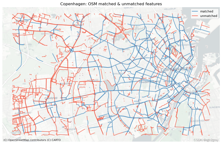
1.2 特征匹配总结
count_matched_osm = len(osm_matched_segments
)
count_matched_ref = len(ref_matched_segments
)perc = np.round(100*count_matched_osm/len(osm_segments), 2)
print(f"Edge count: {count_matched_osm} of {len(osm_segments)} OSM segments ({perc}%) were matched with a reference segment."
)perc = np.round(100*count_matched_ref/len(ref_segments), 2)
print(f"Edge count: {count_matched_ref} out of {len(ref_segments)} {reference_name} segments ({perc}%) were matched with an OSM segment."
)length_matched_osm = osm_matched_segments.geometry.length.sum()length_unmatched_osm = osm_unmatched_segments.geometry.length.sum()length_matched_ref = ref_matched_segments.geometry.length.sum()length_unmatched_ref = ref_unmatched_segments.geometry.length.sum()perc = np.round(100*length_matched_osm/osm_segments.geometry.length.sum() , 2)
print(f"Length: {length_matched_osm/1000:.2f} km out of {osm_segments.geometry.length.sum()/1000:.2f} km of OSM segment ({perc}%) were matched with a reference segment."
)perc = np.round(100*length_matched_ref/ref_segments.geometry.length.sum() , 2)
print(f"Length: {length_matched_ref/1000:.2f} km out of {ref_segments.geometry.length.sum()/1000:.2f} km of {reference_name} segments ({perc}%) were matched with an OSM segment."
)results_feature_matching = {"osm_matched_count": count_matched_osm,"osm_matched_count_pct": count_matched_osm / len(osm_segments) * 100,"ref_matched_count": count_matched_ref,"ref_matched_count_pct": count_matched_ref / len(ref_segments) * 100,"osm_matched_length": length_matched_osm,"osm_matched_length_pct": length_matched_osm/ osm_segments.geometry.length.sum()* 100,"ref_matched_length": length_matched_ref,"ref_matched_length_pct": length_matched_ref/ ref_segments.geometry.length.sum()* 100,
}
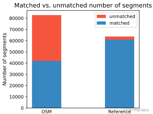
Edge count: 41967 of 82759 OSM segments (50.71%) were matched with a reference segment.
Edge count: 60946 out of 63695 GeoDanmark segments (95.68%) were matched with an OSM segment.
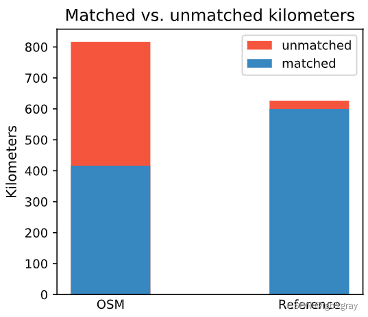
Length: 416.38 km out of 816.70 km of OSM segment (50.98%) were matched with a reference segment.
Length: 599.93 km out of 626.48 km of GeoDanmark segments (95.76%) were matched with an OSM segment.
# Plot matching summaryset_renderer(renderer_plot)# Edges
fig, ax = plt.subplots(1, 1, figsize=pdict["fsbar_small"], sharex=True, sharey=False)
bars = ("OSM", "Reference")
x_pos = [0.5, 1.5]ax.bar(x_pos[0],[len(osm_segments)],width=pdict["bar_single"],color=pdict["nomatch"],label="unmatched",
)
ax.bar(x_pos[0],[count_matched_osm],width=pdict["bar_single"],color=pdict["match"],label="matched",
)ax.bar(x_pos[1],[len(ref_segments)],width=pdict["bar_single"],color=pdict["nomatch"],
)
ax.bar(x_pos[1], [count_matched_ref], width=pdict["bar_single"], color=pdict["match"])ax.set_title("Matched vs. unmatched number of segments")
ax.set_xticks(x_pos, bars)
ax.set_ylabel("Number of segments")
ax.legend()plot_func.save_fig(fig, compare_results_plots_fp + f"matched_unmatched_edges_{buffer_dist}_{hausdorff_threshold}_{angular_threshold}_compare")# Kilometers
fig, ax = plt.subplots(1, 1, figsize=pdict["fsbar_small"], sharex=True, sharey=False)
bars = ("OSM", "Reference")
x_pos = [0.5, 1.5]ax.bar(x_pos[0],[osm_segments.geometry.length.sum() / 1000],width=pdict["bar_single"],color=pdict["nomatch"],label="unmatched",
)
ax.bar(x_pos[0],[length_matched_osm / 1000],width=pdict["bar_single"],color=pdict["match"],label="matched",
)ax.bar(x_pos[1],[ref_segments.geometry.length.sum() / 1000],width=pdict["bar_single"],color=pdict["nomatch"],
)
ax.bar(x_pos[1],[length_matched_ref / 1000],width=pdict["bar_single"],color=pdict["match"],
)ax.set_title("Matched vs. unmatched kilometers")
ax.set_xticks(x_pos, bars)
ax.set_ylabel("Kilometers")ax.legend();plot_func.save_fig(fig, compare_results_plots_fp + f"matched_unmatched_km_{buffer_dist}_{hausdorff_threshold}_{angular_threshold}_compare")
2.分析特征匹配结果
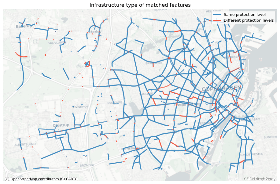
2.1 按基础设施类型匹配的功能
compare_protection = ref_matched_segments[["protected", "geometry", "matches_id", "seg_id_ref"]
].merge(osm_matched_segments[["seg_id", "protected"]],left_on="matches_id",right_on="seg_id",how="inner",suffixes=("_ref", "_osm"),
)assert len(compare_protection) == len(ref_matched_segments)results_feature_matching["protection_level_identical"] = len(compare_protection.loc[compare_protection.protected_ref == compare_protection.protected_osm]
)results_feature_matching["protection_level_differs"] = len(compare_protection.loc[compare_protection.protected_ref != compare_protection.protected_osm]
)
# Plot infrastructure type of matched featuresset_renderer(renderer_map)
fig, ax = plt.subplots(1, 1, figsize=pdict["fsmap"])compare_protection.loc[compare_protection.protected_ref == compare_protection.protected_osm
].plot(ax=ax, color=pdict["match"], linewidth=2, label="Same protection level")compare_protection.loc[compare_protection.protected_ref != compare_protection.protected_osm
].plot(ax=ax, color=pdict["nomatch"], linewidth=2, label="Different protection levels")cx.add_basemap(ax=ax, crs=study_crs, source=cx_tile_2)
ax.set_title("Infrastructure type of matched features")
ax.legend()ax.set_axis_off()plot_func.save_fig(fig,compare_results_static_maps_fp+ f"matched_infra_type_{buffer_dist}_{hausdorff_threshold}_{angular_threshold}_compare",
)
2.2 特征匹配成功
在下图中,总结了每个数据集中匹配和不匹配片段的计数、百分比和长度。
网格单元中的一个数据集中的匹配片段的数量不一定反映另一数据集中的匹配片段的数量,因为片段可以与另一单元中的对应片段匹配。 此外,局部计数是指与网格单元相交的线段。 例如,穿过 2 个单元格的片段将被视为在 2 个不同单元格中匹配。 这不会改变匹配/不匹配片段的相对分布,但它确实需要上面匹配/不匹配片段的总体摘要使用与下面的图不同的片段总数。
# Index ref and osm segments by gridgrid = grid[['grid_id','geometry']]
osm_segments_joined = gpd.overlay(osm_segments[['geometry','seg_id','edge_id']], grid, how="intersection")ref_segments_joined = gpd.overlay(ref_segments[['geometry','seg_id_ref','edge_id']], grid, how="intersection")osm_segments_joined['geom_length'] = osm_segments_joined.geometry.length
ref_segments_joined['geom_length'] = ref_segments_joined.geometry.length# Count features in each grid cell
data = [osm_segments_joined,ref_segments_joined
]
labels = ["osm_segments", "ref_segments"]for data, label in zip(data, labels):df = eval_func.count_features_in_grid(data, label)grid = eval_func.merge_results(grid, df, "left")df = eval_func.length_features_in_grid(data, label)grid = eval_func.merge_results(grid, df, "left")grid['osm_seg_dens'] = grid.length_osm_segments / (grid.area / 1000000)
grid['ref_seg_dens'] = grid.length_ref_segments / (grid.area / 1000000)
# Get matched, joined segments
osm_matched_joined = osm_segments_joined.loc[osm_segments_joined.seg_id.isin(osm_matched_segments.seg_id)
]ref_matched_joined = ref_segments_joined.loc[ref_segments_joined.seg_id_ref.isin(ref_matched_segments.seg_id_ref)
]# Count matched features in each grid cell
data = [osm_matched_joined, ref_matched_joined]
labels = ["osm_matched", "ref_matched"]for data, label in zip(data, labels):df = eval_func.count_features_in_grid(data, label)grid = eval_func.merge_results(grid, df, "left")df = eval_func.length_of_features_in_grid(data, label)grid = eval_func.merge_results(grid, df, "left")# Compute pct matched
grid["pct_matched_osm"] = (grid["count_osm_matched"] / grid["count_osm_segments"] * 100
)
grid["pct_matched_ref"] = (grid["count_ref_matched"] / grid["count_ref_segments"] * 100
)# Compute local min, max, mean of matched
results_feature_matching["osm_pct_matched_local_min"] = grid.pct_matched_osm.min()
results_feature_matching["osm_pct_matched_local_max"] = grid.pct_matched_osm.max()
results_feature_matching["osm_pct_matched_local_mean"] = grid.pct_matched_osm.mean()
results_feature_matching["ref_pct_matched_local_min"] = grid.pct_matched_ref.min()
results_feature_matching["ref_pct_matched_local_max"] = grid.pct_matched_ref.max()
results_feature_matching["ref_pct_matched_local_mean"] = grid.pct_matched_ref.mean()# Compute unmatched
grid.loc[(grid.count_osm_segments.notnull()) & (grid.count_osm_matched.isnull()),["count_osm_matched"],
] = 0
grid.loc[(grid.count_ref_segments.notnull()) & (grid.count_ref_matched.isnull()),["count_ref_matched"],
] = 0
grid.loc[(grid.count_osm_segments.notnull()) & (grid.pct_matched_osm.isnull()),["pct_matched_osm"],
] = 0
grid.loc[(grid.count_ref_segments.notnull()) & (grid.pct_matched_ref.isnull()),["pct_matched_ref"],
] = 0grid.loc[(grid.count_osm_segments.notnull()) & (grid.length_osm_matched.isnull()),["length_osm_matched"],
] = 0
grid.loc[(grid.count_ref_segments.notnull()) & (grid.length_ref_matched.isnull()),["length_ref_matched"],
] = 0grid["count_osm_unmatched"] = grid.count_osm_segments - grid.count_osm_matched
grid["count_ref_unmatched"] = grid.count_ref_segments - grid.count_ref_matchedgrid["length_osm_unmatched"] = grid.length_osm_segments - grid.length_osm_matched
grid["length_ref_unmatched"] = grid.length_ref_segments - grid.length_ref_matched# Compute pct unmatched
grid["pct_unmatched_osm"] = (grid["count_osm_unmatched"] / grid["count_osm_segments"] * 100
)
grid["pct_unmatched_ref"] = (grid["count_ref_unmatched"] / grid["count_ref_segments"] * 100
)grid.loc[grid.pct_matched_osm == 100, "pct_unmatched_osm"] = 0
grid.loc[grid.pct_matched_ref == 100, "pct_unmatched_ref"] = 0
# Plot of matched featuresset_renderer(renderer_map)# Plot count of matched features
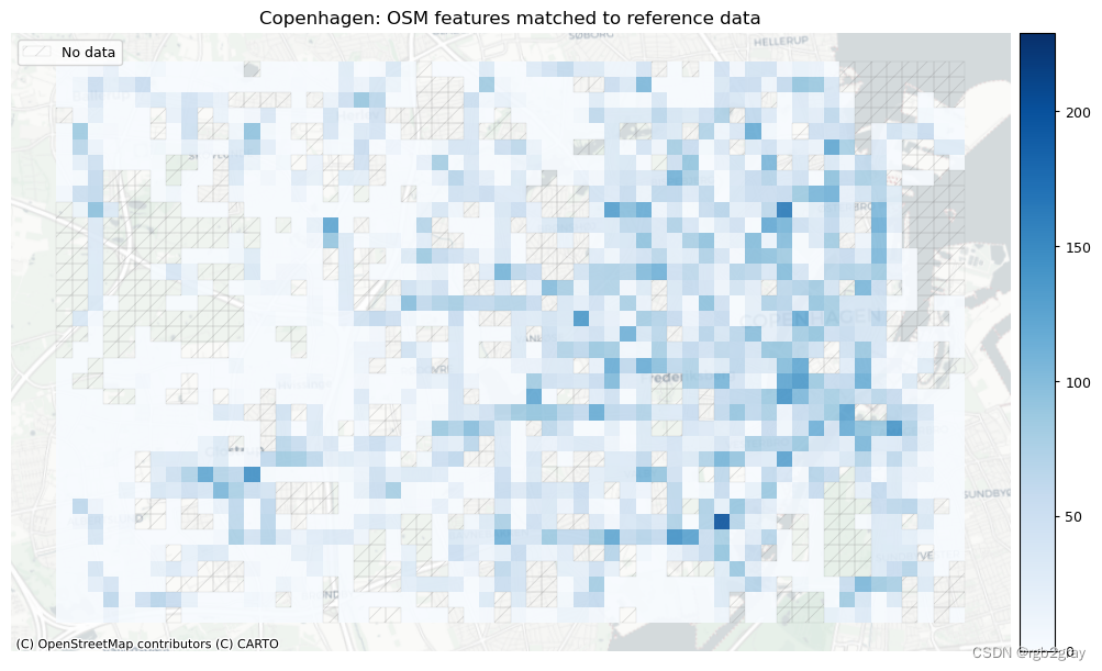
plot_cols = ["count_osm_matched", "count_ref_matched"]
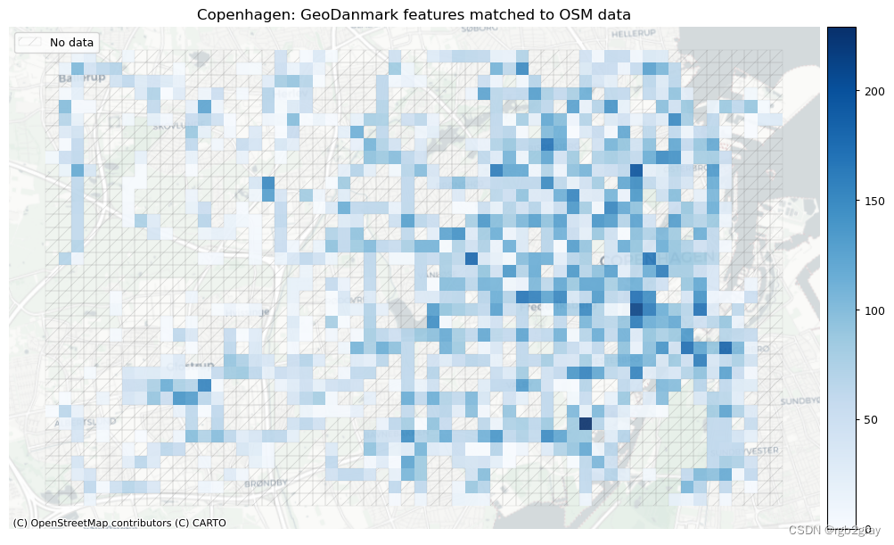
plot_titles = [area_name + ": OSM features matched to reference data",area_name + f": {reference_name} features matched to OSM data",
]
filepaths = [compare_results_static_maps_fp+ f"count_osm_matched_grid_{buffer_dist}_{hausdorff_threshold}_{angular_threshold}_compare",compare_results_static_maps_fp+ f"count_osm_matched_grid_{buffer_dist}_{hausdorff_threshold}_{angular_threshold}_compare",
]
cmaps = [pdict["pos"]] * len(plot_cols)
no_data_cols = ["count_osm_segments", "count_ref_segments"]norm_count_min = [0]*len(plot_cols)
norm_count_max = [grid[["count_osm_matched", "count_ref_matched"]].max().max()]*len(plot_cols)plot_func.plot_grid_results(grid=grid,plot_cols=plot_cols,plot_titles=plot_titles,filepaths=filepaths,cmaps=cmaps,alpha=pdict["alpha_grid"],cx_tile=cx_tile_2,no_data_cols=no_data_cols,use_norm=True,norm_min=norm_count_min,norm_max=norm_count_max,
)# Plot pct of count of matched features
norm_pct_min = [0]*len(plot_cols)
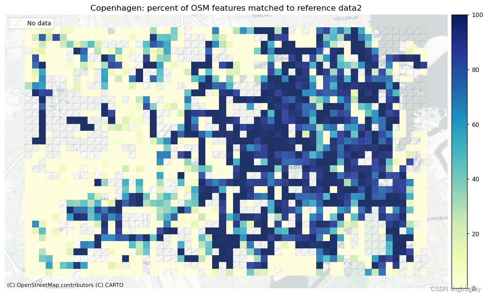
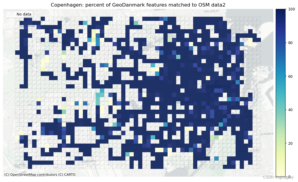
norm_pct_max = [100]*len(plot_cols)plot_cols = ["pct_matched_osm", "pct_matched_ref"]
plot_titles = [area_name + f": percent of OSM features matched to reference data2",area_name + f": percent of {reference_name} features matched to OSM data2",
]
filepaths = [compare_results_static_maps_fp+ f"pct_osm_matched_grid_{buffer_dist}_{hausdorff_threshold}_{angular_threshold}_compare",compare_results_static_maps_fp+ f"pct_ref_matched_grid_{buffer_dist}_{hausdorff_threshold}_{angular_threshold}_compare",
]cmaps = [pdict["seq"]] * len(plot_cols)plot_func.plot_grid_results(grid=grid,plot_cols=plot_cols,plot_titles=plot_titles,filepaths=filepaths,cmaps=cmaps,alpha=pdict["alpha_grid"],cx_tile=cx_tile_2,no_data_cols=no_data_cols,use_norm=True,norm_min=norm_pct_min,norm_max=norm_pct_max,
)# Plot length of matched features
norm_length_min = [0]*len(plot_cols)
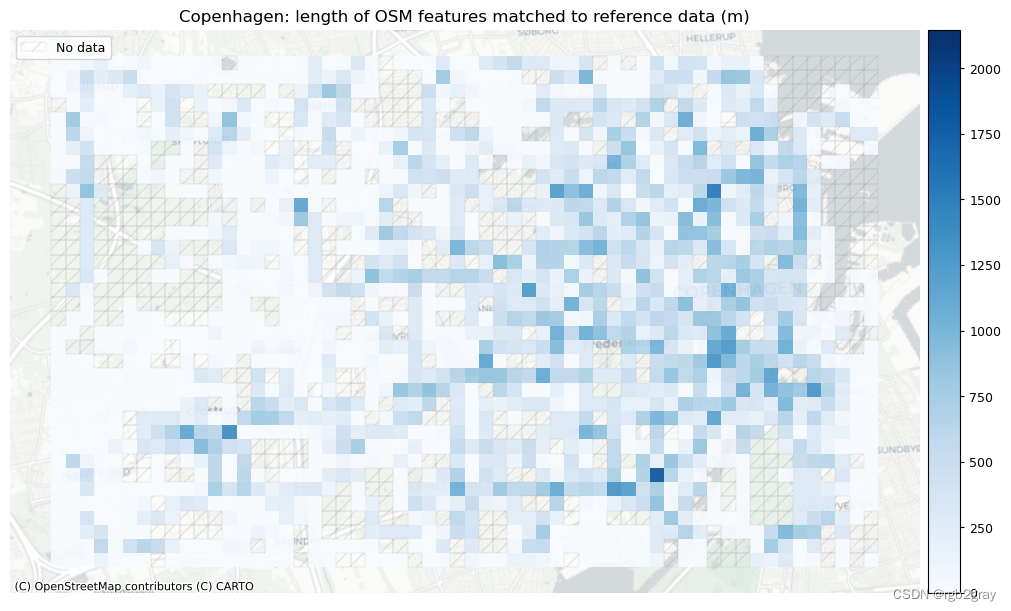
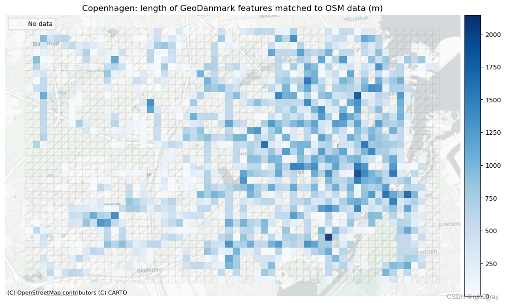
norm_length_max = [grid[["length_osm_matched", "length_ref_matched"]].max().max()]*len(plot_cols)plot_cols = ["length_osm_matched", "length_ref_matched"]
plot_titles = [area_name + f": length of OSM features matched to reference data (m)",area_name + f": length of {reference_name} features matched to OSM data (m)",
]
filepaths = [compare_results_static_maps_fp+ f"length_osm_matched_grid_{buffer_dist}_{hausdorff_threshold}_{angular_threshold}_compare",compare_results_static_maps_fp+ f"length_ref_matched_grid_{buffer_dist}_{hausdorff_threshold}_{angular_threshold}_compare",
]cmaps = [pdict["pos"]] * len(plot_cols)plot_func.plot_grid_results(grid=grid,plot_cols= plot_cols,plot_titles=plot_titles,filepaths=filepaths,cmaps=cmaps,alpha=pdict["alpha_grid"],cx_tile=cx_tile_2,no_data_cols=no_data_cols,use_norm=True,norm_min=norm_length_min,norm_max=norm_length_max,
)
# Plot of unmatched featuresset_renderer(renderer_map)cmaps = [pdict["neg"]] * len(plot_cols)
no_data_cols = ["count_osm_segments", "count_ref_segments"]# Plot count of matched features
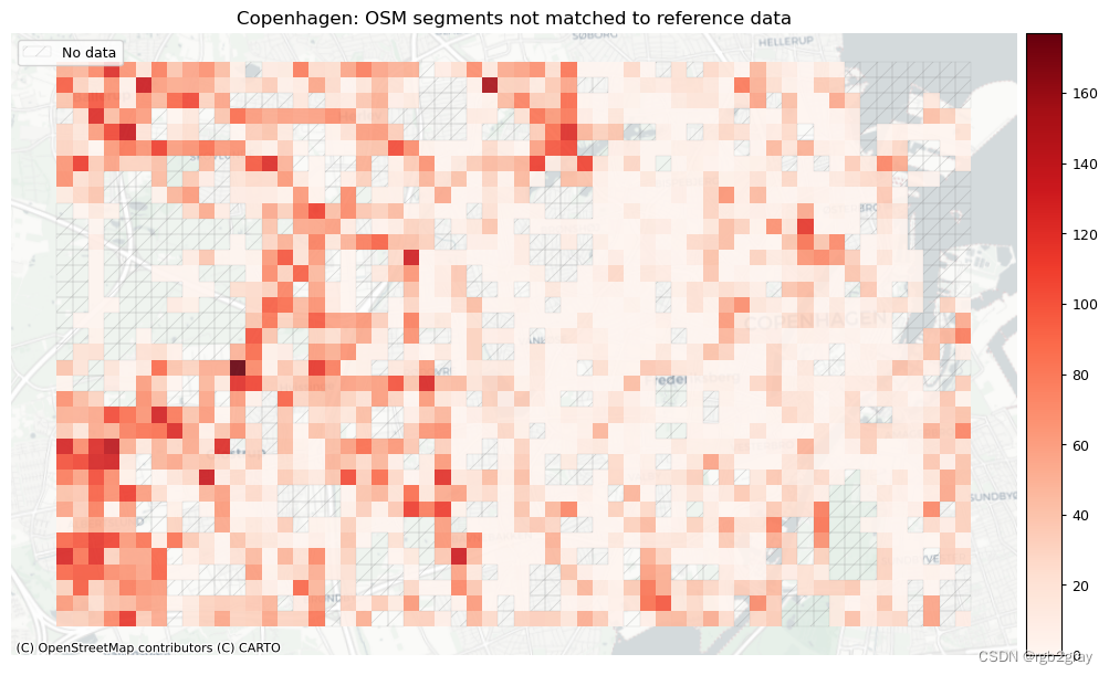
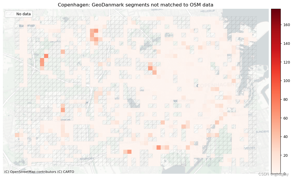
plot_cols = ["count_osm_unmatched", "count_ref_unmatched"]
plot_titles = [area_name + f": OSM segments not matched to reference data",area_name + f": {reference_name} segments not matched to OSM data",
]
filepaths = [compare_results_static_maps_fp+ f"count_osm_unmatched_grid_{buffer_dist}_{hausdorff_threshold}_{angular_threshold}_compare",compare_results_static_maps_fp+ f"count_osm_unmatched_grid_{buffer_dist}_{hausdorff_threshold}_{angular_threshold}_compare",
]norm_count_min = [0]*len(plot_cols)
norm_count_max = [grid[["count_osm_unmatched", "count_ref_unmatched"]].max().max()]*len(plot_cols)plot_func.plot_grid_results(grid=grid,plot_cols=plot_cols,plot_titles=plot_titles,filepaths=filepaths,cmaps=cmaps,alpha=pdict["alpha_grid"],cx_tile=cx_tile_2,no_data_cols=no_data_cols,use_norm=True,norm_min=norm_count_min,norm_max=norm_count_max,
)# Plot pct of count of matched segments
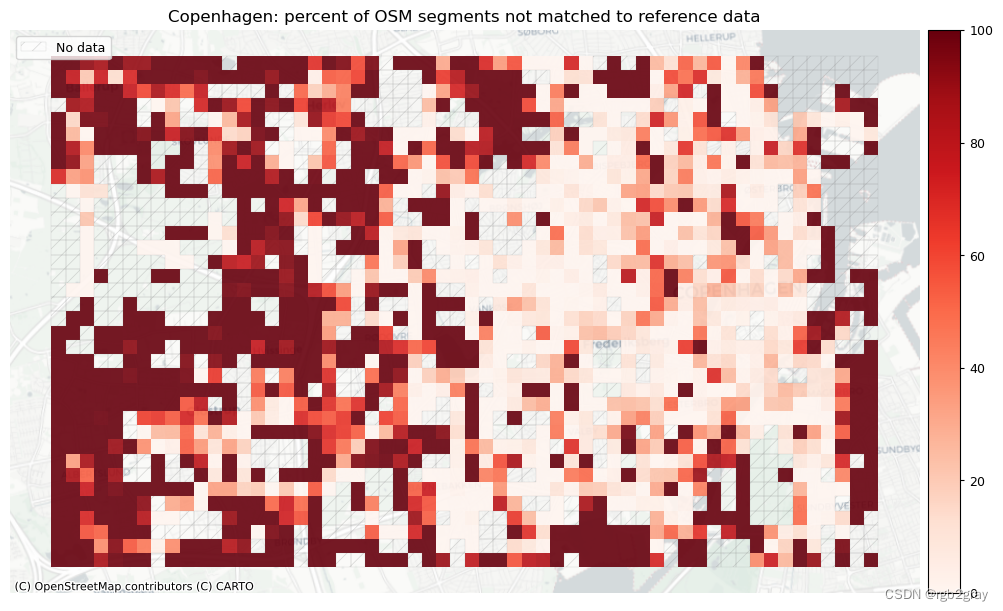
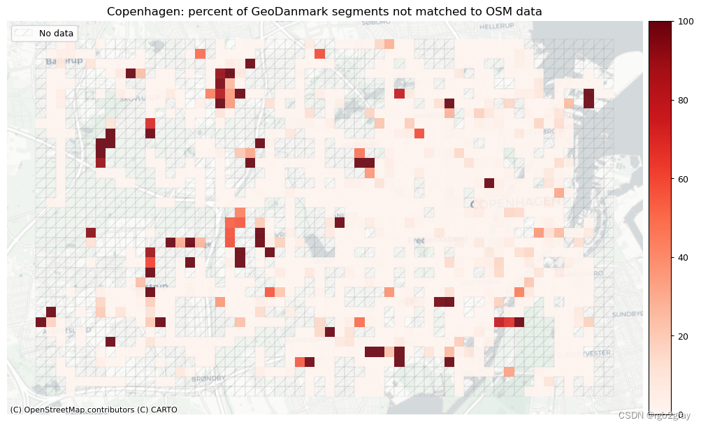
plot_cols = ["pct_unmatched_osm", "pct_unmatched_ref"]
plot_titles = [area_name + ": percent of OSM segments not matched to reference data",area_name + f": percent of {reference_name} segments not matched to OSM data",
]
filepaths = [compare_results_static_maps_fp+ f"pct_osm_unmatched_grid_{buffer_dist}_{hausdorff_threshold}_{angular_threshold}_compare",compare_results_static_maps_fp+ f"pct_ref_unmatched_grid_{buffer_dist}_{hausdorff_threshold}_{angular_threshold}_compare",
]norm_pct_min = [0]*len(plot_cols)
norm_pct_max = [100]*len(plot_cols)plot_func.plot_grid_results(grid=grid,plot_cols=plot_cols,plot_titles=plot_titles,filepaths=filepaths,cmaps=cmaps,alpha=pdict["alpha_grid"],cx_tile=cx_tile_2,no_data_cols=no_data_cols,use_norm=True,norm_min=norm_pct_min,norm_max=norm_pct_max,
)# Plot length of matched segments
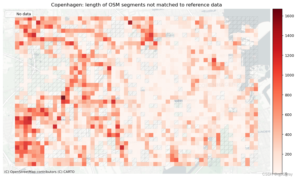
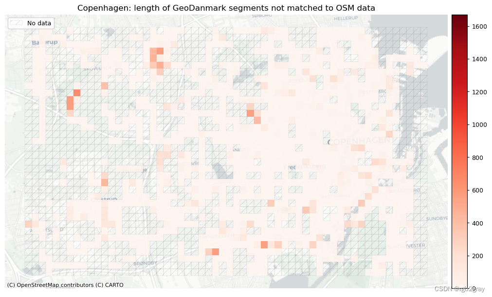
plot_cols = ["length_osm_unmatched", "length_ref_unmatched"]
plot_titles = [area_name + ": length of OSM segments not matched to reference data",area_name + f": length of {reference_name} segments not matched to OSM data",
]
filepaths = [compare_results_static_maps_fp+ f"length_osm_unmatched_grid_{buffer_dist}_{hausdorff_threshold}_{angular_threshold}_compare",compare_results_static_maps_fp+ f"length_ref_unmatched_grid_{buffer_dist}_{hausdorff_threshold}_{angular_threshold}_compare",
]norm_length_min = [0]*len(plot_cols)
norm_length_max = [grid[["length_osm_unmatched", "length_ref_unmatched"]].max().max()]*len(plot_cols)plot_func.plot_grid_results(grid=grid,plot_cols=plot_cols,plot_titles=plot_titles,filepaths=filepaths,cmaps=cmaps,alpha=pdict["alpha_grid"],cx_tile=cx_tile_2,no_data_cols=no_data_cols,use_norm=True,norm_min=norm_length_min,norm_max=norm_length_max,
)
3. 概括
osm_keys = [x for x in results_feature_matching.keys() if "osm" in x]
ref_keys = [x for x in results_feature_matching.keys() if "ref" in x]osm_values = [results_feature_matching[x] for x in osm_keys]
osm_df = pd.DataFrame(osm_values, index=osm_keys)osm_df.rename({0: "OSM"}, axis=1, inplace=True)# Convert to km
osm_df.loc["osm_matched_length"] = osm_df.loc["osm_matched_length"] / 1000rename_metrics = {"osm_matched_count": "Count of matched segments","osm_matched_count_pct": "Percent matched segments","osm_matched_length": "Length of matched segments (km)","osm_matched_length_pct": "Percent of matched network length","osm_pct_matched_local_min": "Local min of % matched segments","osm_pct_matched_local_max": "Local max of % matched segments","osm_pct_matched_local_mean": "Local average of % matched segments",
}osm_df.rename(rename_metrics, inplace=True)ref_keys = [x for x in results_feature_matching.keys() if "ref" in x]ref_values = [results_feature_matching[x] for x in ref_keys]
ref_df = pd.DataFrame(ref_values, index=ref_keys)# Convert to km
ref_df.loc["ref_matched_length"] = ref_df.loc["ref_matched_length"] / 1000ref_df.rename({0: reference_name}, axis=1, inplace=True)rename_metrics = {"ref_matched_count": "Count of matched segments","ref_matched_count_pct": "Percent matched segments","ref_matched_length": "Length of matched segments (km)","ref_matched_length_pct": "Percent of matched network length","ref_pct_matched_local_min": "Local min of % matched segments","ref_pct_matched_local_max": "Local max of % matched segments","ref_pct_matched_local_mean": "Local average of % matched segments",
}ref_df.rename(rename_metrics, inplace=True)
combined_results = pd.concat([osm_df, ref_df], axis=1)combined_results.style.pipe(format_matched_style)
D:\tmp_resource\BikeDNA-main\BikeDNA-main\scripts\settings\df_styler.py:133: FutureWarning: Styler.applymap_index has been deprecated. Use Styler.map_index instead.styler.applymap_index(
| OSM | GeoDanmark | |
|---|---|---|
| Count of matched segments | 41,967 | 60,946 |
| Percent matched segments | 51% | 96% |
| Length of matched segments (km) | 416 | 600 |
| Percent of matched network length | 51% | 96% |
| Local min of % matched segments | 1% | 2% |
| Local max of % matched segments | 100% | 100% |
| Local average of % matched segments | 73% | 96% |
# Export to CSVcombined_results.to_csv(compare_results_data_fp + "feature_matching_summary_stats.csv", index=True
)
4. 保存结果
with open(f"../../results/compare/{study_area}/data/feature_matches__{buffer_dist}_{hausdorff_threshold}_{angular_threshold}.json","w",
) as outfile:json.dump(results_feature_matching, outfile)with open(f"../../results/compare/{study_area}/data/grid_results_feature_matching_{buffer_dist}_{hausdorff_threshold}_{angular_threshold}.pickle","wb",
) as f:pickle.dump(grid, f)
from time import strftime
print("Time of analysis: " + strftime("%a, %d %b %Y %H:%M:%S"))
Time of analysis: Mon, 18 Dec 2023 20:41:52
相关文章:
BikeDNA(九) 特征匹配
BikeDNA(九) 特征匹配 特征匹配采用参考数据并尝试识别 OSM 数据集中的相应特征。 特征匹配是比较单个特征而不是研究区域网格单元水平上的特征特征的必要前提。 方法 将两个道路数据集中的特征与其数字化特征的方式以及边缘之间潜在的一对多关系进行…...

vuex是什么?怎么使用?哪种功能场景使用它?
Vuex是Vue.js官方推荐的状态管理库,用于在Vue应用程序中管理和共享状态。它基于Flux架构和单向数据流的概念,将应用程序的状态集中管理,使得状态的变化更可追踪、更易于管理。Vuex提供了一个全局的状态树,以及一些用于修改状态的方…...
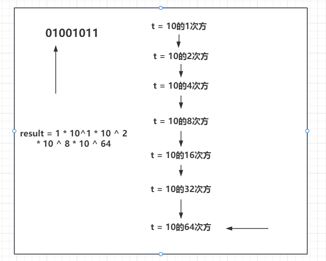
求斐波那契数列矩阵乘法的方法
斐波那契数列 先来简单介绍一下斐波那契数列: 斐波那契数列是指这样一个数列:1,1,2,3,5,8,13,21,34,55,89……这个数列从第3项开始 &…...
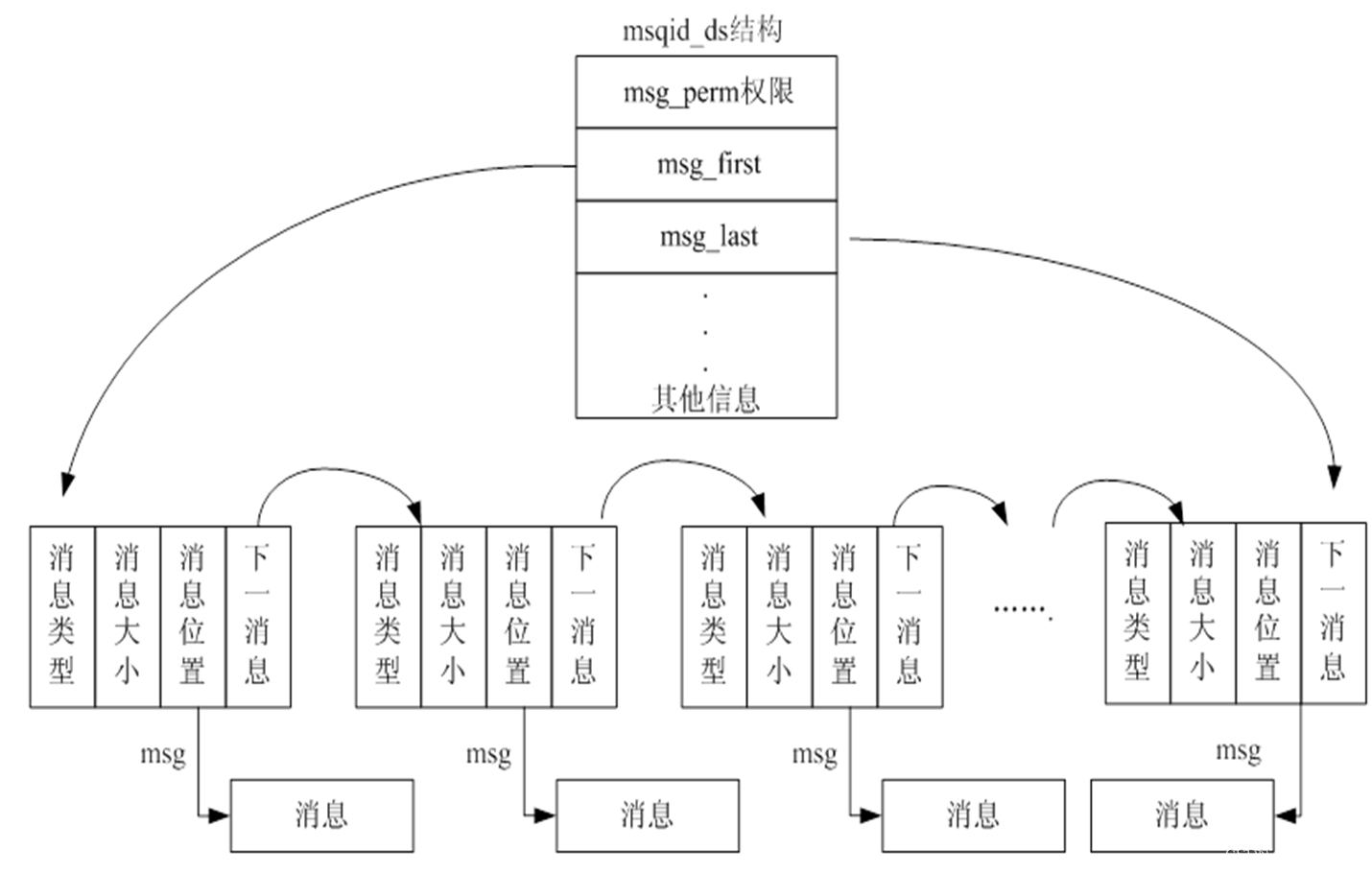
【IPC通信--消息队列】
消息队列(也叫做报文队列)是一个消息的链表。可以把消息看作一个记录,具有特定的格式以及特定的优先级。对消息队列有写权限的进程可以向消息队列中按照一定的规则添加新消息;对消息队列有读权限的进程则可以从消息队列中读走消息…...
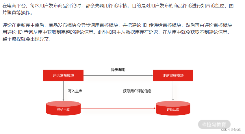
读写分离的手段——主从复制,解决读流量大大高于写流量的问题
应用场景 假设说有这么一种业务场景,读流量显著高于写流量,你要怎么优化呢。因为写是要加锁的,可能就会阻塞你读请求。而且其实读多写少的场景还很多见,比如电商平台,用户浏览n多个商品才会买一个。 大部分人的思路可…...
Day02
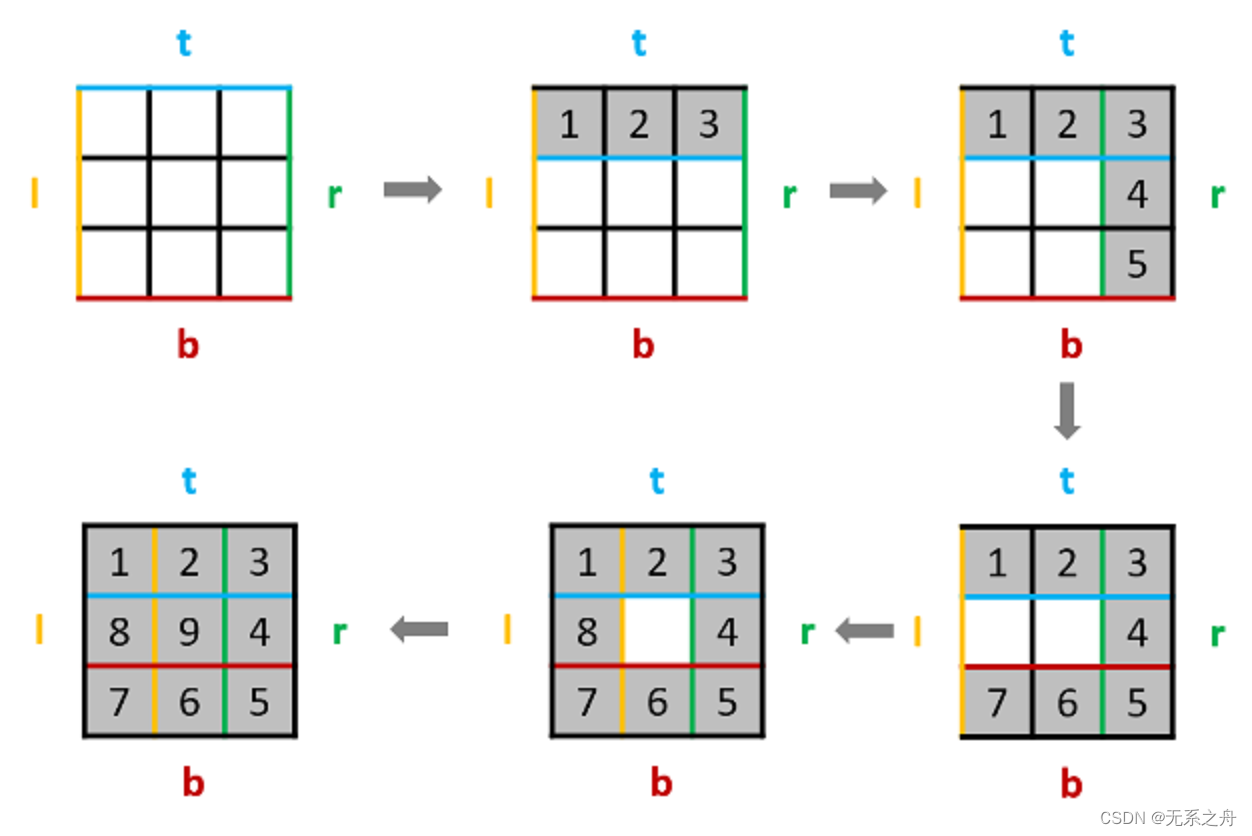
今日任务: 977 有序数组的平方209 长度最小的子数组59 螺旋矩阵Ⅱ 977 有序数组的平方 题目链接:https://leetcode.cn/problems/squares-of-a-sorted-array/ 双指针问题,以及数组本身时有序的; 思路: 左、右两个…...

编程语言的发展未来?
编程语言的未来? 随着科技的飞速发展,编程语言在计算机领域中扮演着至关重要的角色。它们是软件开发的核心,为程序员提供了与机器沟通的桥梁。那么,在技术不断进步的未来,编程语言的走向又将如何呢? 方向…...

docsify阿里云上部署
使用Markdown格式安装和部署Nginx 本文将介绍如何使用Markdown格式安装和部署Nginx。 步骤 安装Nginx: 打开终端,并根据您的操作系统执行以下命令来安装Nginx: 对于Ubuntu或Debian系统: sudo apt-get update sudo apt-get insta…...

GPT实战系列-简单聊聊LangChain搭建本地知识库准备
GPT实战系列-简单聊聊LangChain搭建本地知识库准备 LangChain 是一个开发由语言模型驱动的应用程序的框架,除了和应用程序通过 API 调用, 还会: 数据感知 : 将语言模型连接到其他数据源 具有代理性质 : 允许语言模型与其环境交互 LLM大模型…...

[NAND Flash 6.4] NAND FLASH基本读操作及原理_NAND FLASH Read Operation源码实现
依公知及经验整理,原创保护,禁止转载。 专栏 《深入理解NAND Flash》 <<<< 返回总目录 <<<< 全文 6000 字 内容摘要 NAND Flash 引脚功能 读操作步骤 NAND Flash中的特殊硬件结构 NAND Flash 读写时的数据流向 Read 操作时序 读时序操作过…...

opencv多张图片实现全景拼接
最近camera项目需要用到全景拼接,故此查阅大量资料,终于将此功能应用在实际项目上,下面总结一下此过程中遇到的一些问题及解决方式,同时也会将源码附在结尾处,供大家参考,本文采用的opencv版本为3.4.12。 首…...

深入理解UML中的继承关系
深入理解UML中的继承关系 在面向对象的设计中,继承关系是构建清晰、可维护系统的关键。统一建模语言(UML)提供了一种标准化的方法来可视化这些关系。本文将深入探讨UML中的继承关系,并探讨它如何在代码中体现。 什么是继承关系&a…...
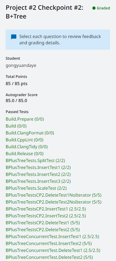
CMU15-445-Spring-2023-Project #2 - B+Tree
前置知识:参考上一篇博文 CMU15-445-Spring-2023-Project #2 - 前置知识(lec07-010) CHECKPOINT #1 Task #1 - BTree Pages 实现三个page class来存储B树的数据。 BTree Page internal page和leaf page继承的基类,只包含两个…...
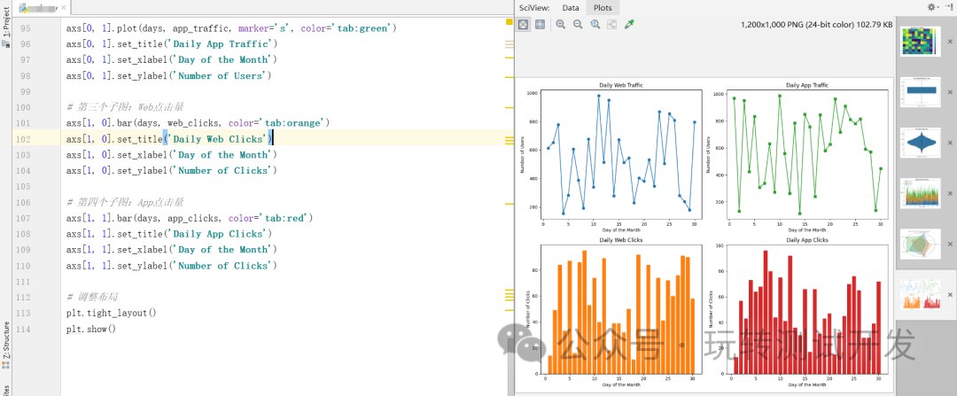
matplotlib:热图、箱形图、小提琴图、堆叠面积图、雷达图、子图
简介:在数字化的世界里,从Web、HTTP到App,数据无处不在。但如何将这些复杂的数据转化为直观、易懂的信息?本文将介绍六种数据可视化方法,帮助你更好地理解和呈现数据。 热图 (Heatmap):热图能有效展示用户…...
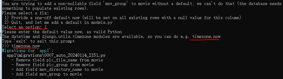
Django数据库选移的preserve_default=False是什么意思?
有下面的迁移命令: migrations.AddField(model_namemovie,namemov_group,fieldmodels.CharField(defaultdjango.utils.timezone.now, max_length30),preserve_defaultFalse,),迁移命令中的preserve_defaultFalse是什么意思呢? 答:如果模型定…...

逸学Docker【java工程师基础】2.Docker镜像容器基本操作+安装MySQL镜像运行
基础的镜像操作 在这里我们的应用程序比如redis需要构建成镜像,它作为一个Docker文件就可以进行构建,构建完以后他是在本地的,我们可以推送到镜像服务器,逆向可以拉取到上传的镜像,或者说我们可以保存为压缩包进行相互…...

基于Java SSM框架实现医院管理系统项目【项目源码】计算机毕业设计
基于java的SSM框架实现医院管理系统演示 SSM框架 当今流行的“SSM组合框架”是Spring SpringMVC MyBatis的缩写,受到很多的追捧,“组合SSM框架”是强强联手、各司其职、协调互补的团队精神。web项目的框架,通常更简单的数据源。Spring属于…...
【java八股文】之Spring系列篇
【java八股文】之JVM基础篇-CSDN博客 【java八股文】之MYSQL基础篇-CSDN博客 【java八股文】之Redis基础篇-CSDN博客 【java八股文】之Spring系列篇-CSDN博客 【java八股文】之分布式系列篇-CSDN博客 【java八股文】之多线程篇-CSDN博客 【java八股文】之JVM基础篇-CSDN博…...

关于MySQL源码的学习 这里是一些建议
学习MySQL源码需要一定的编程基础,特别是C语言和数据结构。以下是一些建议,帮助你更好地入手学习MySQL源码: 基础知识 熟悉C语言编程基本概念、数据结构和算法。了解Linux操作系统基本概念,如进程、线程、内存管理、文件系统等。…...
Mysql是怎样运行的--下
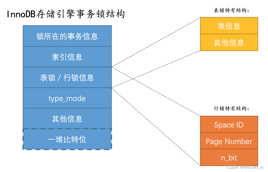
文章目录 Mysql是怎样运行的--下查询优化explainoptimizer_trace InnoDB的Buffer Pool(缓冲池)Buffer Pool的存储结构空闲页存储--free链表脏页(修改后的数据)存储--flush链表 使用Buffer PoolLRU链表的管理 事务ACID事务的状态事…...

铭豹扩展坞 USB转网口 突然无法识别解决方法
当 USB 转网口扩展坞在一台笔记本上无法识别,但在其他电脑上正常工作时,问题通常出在笔记本自身或其与扩展坞的兼容性上。以下是系统化的定位思路和排查步骤,帮助你快速找到故障原因: 背景: 一个M-pard(铭豹)扩展坞的网卡突然无法识别了,扩展出来的三个USB接口正常。…...

【网络】每天掌握一个Linux命令 - iftop
在Linux系统中,iftop是网络管理的得力助手,能实时监控网络流量、连接情况等,帮助排查网络异常。接下来从多方面详细介绍它。 目录 【网络】每天掌握一个Linux命令 - iftop工具概述安装方式核心功能基础用法进阶操作实战案例面试题场景生产场景…...
XCTF-web-easyupload
试了试php,php7,pht,phtml等,都没有用 尝试.user.ini 抓包修改将.user.ini修改为jpg图片 在上传一个123.jpg 用蚁剑连接,得到flag...
VB.net复制Ntag213卡写入UID
本示例使用的发卡器:https://item.taobao.com/item.htm?ftt&id615391857885 一、读取旧Ntag卡的UID和数据 Private Sub Button15_Click(sender As Object, e As EventArgs) Handles Button15.Click轻松读卡技术支持:网站:Dim i, j As IntegerDim cardidhex, …...

3.3.1_1 检错编码(奇偶校验码)
从这节课开始,我们会探讨数据链路层的差错控制功能,差错控制功能的主要目标是要发现并且解决一个帧内部的位错误,我们需要使用特殊的编码技术去发现帧内部的位错误,当我们发现位错误之后,通常来说有两种解决方案。第一…...

FastAPI 教程:从入门到实践
FastAPI 是一个现代、快速(高性能)的 Web 框架,用于构建 API,支持 Python 3.6。它基于标准 Python 类型提示,易于学习且功能强大。以下是一个完整的 FastAPI 入门教程,涵盖从环境搭建到创建并运行一个简单的…...

【ROS】Nav2源码之nav2_behavior_tree-行为树节点列表
1、行为树节点分类 在 Nav2(Navigation2)的行为树框架中,行为树节点插件按照功能分为 Action(动作节点)、Condition(条件节点)、Control(控制节点) 和 Decorator(装饰节点) 四类。 1.1 动作节点 Action 执行具体的机器人操作或任务,直接与硬件、传感器或外部系统…...

Android Bitmap治理全解析:从加载优化到泄漏防控的全生命周期管理
引言 Bitmap(位图)是Android应用内存占用的“头号杀手”。一张1080P(1920x1080)的图片以ARGB_8888格式加载时,内存占用高达8MB(192010804字节)。据统计,超过60%的应用OOM崩溃与Bitm…...

【碎碎念】宝可梦 Mesh GO : 基于MESH网络的口袋妖怪 宝可梦GO游戏自组网系统
目录 游戏说明《宝可梦 Mesh GO》 —— 局域宝可梦探索Pokmon GO 类游戏核心理念应用场景Mesh 特性 宝可梦玩法融合设计游戏构想要素1. 地图探索(基于物理空间 广播范围)2. 野生宝可梦生成与广播3. 对战系统4. 道具与通信5. 延伸玩法 安全性设计 技术选…...
基础)
6个月Python学习计划 Day 16 - 面向对象编程(OOP)基础
第三周 Day 3 🎯 今日目标 理解类(class)和对象(object)的关系学会定义类的属性、方法和构造函数(init)掌握对象的创建与使用初识封装、继承和多态的基本概念(预告) &a…...