R可视化:ggpubr包学习
欢迎大家关注全网生信学习者系列:
-
WX公zhong号:生信学习者
-
Xiao hong书:生信学习者
-
知hu:生信学习者
-
CDSN:生信学习者2
介绍
ggpubr是我经常会用到的R包,它傻瓜式的画图方式对很多初次接触R绘图的人来讲是很友好的。该包有个stat_compare_means函数可以做组间假设检验分析。
安装R包
install.packages("ggpubr")
devtools::devtools::install_github("kassambara/ggpubr")
library(ggpubr)
plotdata <- data.frame(sex = factor(rep(c("F", "M"), each=200)),weight = c(rnorm(200, 55), rnorm(200, 58)))
密度图density
ggdensity(plotdata, x = "weight",add = "mean", rug = TRUE, # x轴显示分布密度color = "sex", fill = "sex",palette = c("#00AFBB", "#E7B800"))

柱状图histogram
gghistogram(plotdata, x = "weight",bins = 30,add = "mean", rug = TRUE,color = "sex", fill = "sex",palette = c("#00AFBB", "#E7B800"))

箱线图boxplot
df <- ToothGrowth
head(df)
my_comparisons <- list( c("0.5", "1"), c("1", "2"), c("0.5", "2") )
ggboxplot(df, x = "dose", y = "len",color = "dose", palette =c("#00AFBB", "#E7B800", "#FC4E07"),add = "jitter", shape = "dose")+stat_compare_means(comparisons = my_comparisons)+ # Add pairwise comparisons p-valuestat_compare_means(label.y = 50)

小提琴图violin
ggviolin(df, x = "dose", y = "len", fill = "dose",palette = c("#00AFBB", "#E7B800", "#FC4E07"),add = "boxplot", add.params = list(fill = "white"))+stat_compare_means(comparisons = my_comparisons, label = "p.signif")+ # Add significance levelsstat_compare_means(label.y = 50)

点图dotplot
ggdotplot(ToothGrowth, x = "dose", y = "len",color = "dose", palette = "jco", binwidth = 1)

有序条形图 ordered bar plots
data("mtcars")
dfm <- mtcars
dfm$cyl <- as.factor(dfm$cyl)
dfm$name <- rownames(dfm)
head(dfm[, c("name", "wt", "mpg", "cyl")])
ggbarplot(dfm, x = "name", y = "mpg",fill = "cyl", # change fill color by cylcolor = "white", # Set bar border colors to whitepalette = "jco", # jco journal color palett. see ?ggparsort.val = "asc", # Sort the value in dscending ordersort.by.groups = TRUE, # Sort inside each groupx.text.angle = 90) # Rotate vertically x axis texts

偏差图Deviation graphs
dfm$mpg_z <- (dfm$mpg -mean(dfm$mpg))/sd(dfm$mpg)
dfm$mpg_grp <- factor(ifelse(dfm$mpg_z < 0, "low", "high"), levels = c("low", "high"))
# Inspect the data
head(dfm[, c("name", "wt", "mpg", "mpg_z", "mpg_grp", "cyl")])
ggbarplot(dfm, x = "name", y = "mpg_z",fill = "mpg_grp", # change fill color by mpg_levelcolor = "white", # Set bar border colors to whitepalette = "jco", # jco journal color palett. see ?ggparsort.val = "asc", # Sort the value in ascending ordersort.by.groups = FALSE, # Don't sort inside each groupx.text.angle = 90, # Rotate vertically x axis textsylab = "MPG z-score",rotate = FALSE,xlab = FALSE,legend.title = "MPG Group")

棒棒糖图 lollipop chart
ggdotchart(dfm, x = "name", y = "mpg",color = "cyl", # Color by groupspalette = c("#00AFBB", "#E7B800", "#FC4E07"), # Custom color palettesorting = "descending", # Sort value in descending orderadd = "segments", # Add segments from y = 0 to dotsrotate = TRUE, # Rotate verticallygroup = "cyl", # Order by groupsdot.size = 6, # Large dot sizelabel = round(dfm$mpg), # Add mpg values as dot labelsfont.label = list(color = "white", size = 9, vjust = 0.5), # Adjust label parametersggtheme = theme_pubr()) # ggplot2 theme

偏差图Deviation graph
ggdotchart(dfm, x = "name", y = "mpg_z",color = "cyl", # Color by groupspalette = c("#00AFBB", "#E7B800", "#FC4E07"), # Custom color palettesorting = "descending", # Sort value in descending orderadd = "segments", # Add segments from y = 0 to dotsadd.params = list(color = "lightgray", size = 2), # Change segment color and sizegroup = "cyl", # Order by groupsdot.size = 6, # Large dot sizelabel = round(dfm$mpg_z,1), # Add mpg values as dot labelsfont.label = list(color = "white", size = 9, vjust = 0.5), # Adjust label parametersggtheme = theme_pubr())+ # ggplot2 themegeom_hline(yintercept = 0, linetype = 2, color = "lightgray")

散点图scatterplot
df <- datasets::iris
head(df)
ggscatter(df, x = 'Sepal.Width', y = 'Sepal.Length', palette = 'jco', shape = 'Species', add = 'reg.line',color = 'Species', conf.int = TRUE)

-
添加回归线的系数
ggscatter(df, x = 'Sepal.Width', y = 'Sepal.Length', palette = 'jco', shape = 'Species', add = 'reg.line',color = 'Species', conf.int = TRUE)+stat_cor(aes(color=Species),method = "pearson", label.x = 3)

-
添加聚类椭圆 concentration ellipses
data("mtcars")
dfm <- mtcars
dfm$cyl <- as.factor(dfm$cyl)
dfm$name <- rownames(dfm)
p1 <- ggscatter(dfm, x = "wt", y = "mpg",color = "cyl", palette = "jco",shape = "cyl",ellipse = TRUE)
p2 <- ggscatter(dfm, x = "wt", y = "mpg",color = "cyl", palette = "jco",shape = "cyl",ellipse = TRUE,ellipse.type = "convex")
cowplot::plot_grid(p1, p2, align = "hv", nrow = 1)

-
添加mean和stars
ggscatter(dfm, x = "wt", y = "mpg",color = "cyl", palette = "jco",shape = "cyl",ellipse = TRUE, mean.point = TRUE,star.plot = TRUE)

-
显示点标签
dfm$name <- rownames(dfm)
p3 <- ggscatter(dfm, x = "wt", y = "mpg",color = "cyl", palette = "jco",label = "name",repel = TRUE)
p4 <- ggscatter(dfm, x = "wt", y = "mpg",color = "cyl", palette = "jco",label = "name",repel = TRUE,label.select = c("Toyota Corolla", "Merc 280", "Duster 360"))
cowplot::plot_grid(p3, p4, align = "hv", nrow = 1)

气泡图bubble plot
ggscatter(dfm, x = "wt", y = "mpg",color = "cyl",palette = "jco",size = "qsec", alpha = 0.5)+scale_size(range = c(0.5, 15)) # Adjust the range of points size

连线图 lineplot
p1 <- ggbarplot(ToothGrowth, x = "dose", y = "len", add = "mean_se",color = "supp", palette = "jco", position = position_dodge(0.8))+stat_compare_means(aes(group = supp), label = "p.signif", label.y = 29)
p2 <- ggline(ToothGrowth, x = "dose", y = "len", add = "mean_se",color = "supp", palette = "jco")+stat_compare_means(aes(group = supp), label = "p.signif", label.y = c(16, 25, 29))
cowplot::plot_grid(p1, p2, ncol = 2, align = "hv")

添加边沿图 marginal plots
library(ggExtra)
p <- ggscatter(iris, x = "Sepal.Length", y = "Sepal.Width",color = "Species", palette = "jco",size = 3, alpha = 0.6)
ggMarginal(p, type = "boxplot")

-
第二种添加方式: 分别画出三个图,然后进行组合
sp <- ggscatter(iris, x = "Sepal.Length", y = "Sepal.Width",color = "Species", palette = "jco",size = 3, alpha = 0.6, ggtheme = theme_bw())
xplot <- ggboxplot(iris, x = "Species", y = "Sepal.Length", color = "Species", fill = "Species", palette = "jco",alpha = 0.5, ggtheme = theme_bw())+ rotate()
yplot <- ggboxplot(iris, x = "Species", y = "Sepal.Width",color = "Species", fill = "Species", palette = "jco",alpha = 0.5, ggtheme = theme_bw())
sp <- sp + rremove("legend")
yplot <- yplot + clean_theme() + rremove("legend")
xplot <- xplot + clean_theme() + rremove("legend")
cowplot::plot_grid(xplot, NULL, sp, yplot, ncol = 2, align = "hv", rel_widths = c(2, 1), rel_heights = c(1, 2))

-
上图主图和边沿图之间的space太大,第三种方法能克服这个缺点
library(cowplot)
# Main plot
pmain <- ggplot(iris, aes(x = Sepal.Length, y = Sepal.Width, color = Species))+geom_point()+ggpubr::color_palette("jco")
# Marginal densities along x axis
xdens <- axis_canvas(pmain, axis = "x")+geom_density(data = iris, aes(x = Sepal.Length, fill = Species),alpha = 0.7, size = 0.2)+ggpubr::fill_palette("jco")
# Marginal densities along y axis
# Need to set coord_flip = TRUE, if you plan to use coord_flip()
ydens <- axis_canvas(pmain, axis = "y", coord_flip = TRUE)+geom_boxplot(data = iris, aes(x = Sepal.Width, fill = Species),alpha = 0.7, size = 0.2)+coord_flip()+ggpubr::fill_palette("jco")
p1 <- insert_xaxis_grob(pmain, xdens, grid::unit(.2, "null"), position = "top")
p2 <- insert_yaxis_grob(p1, ydens, grid::unit(.2, "null"), position = "right")
ggdraw(p2)

-
第四种方法,通过grob设置
# Scatter plot colored by groups ("Species")
#::::::::::::::::::::::::::::::::::::::::::::::::::::::::::
sp <- ggscatter(iris, x = "Sepal.Length", y = "Sepal.Width",color = "Species", palette = "jco",size = 3, alpha = 0.6)
# Create box plots of x/y variables
#::::::::::::::::::::::::::::::::::::::::::::::::::::::::::
# Box plot of the x variable
xbp <- ggboxplot(iris$Sepal.Length, width = 0.3, fill = "lightgray") +rotate() +theme_transparent()
# Box plot of the y variable
ybp <- ggboxplot(iris$Sepal.Width, width = 0.3, fill = "lightgray") +theme_transparent()
# Create the external graphical objects
# called a "grop" in Grid terminology
xbp_grob <- ggplotGrob(xbp)
ybp_grob <- ggplotGrob(ybp)
# Place box plots inside the scatter plot
#::::::::::::::::::::::::::::::::::::::::::::::::::::::::::
xmin <- min(iris$Sepal.Length); xmax <- max(iris$Sepal.Length)
ymin <- min(iris$Sepal.Width); ymax <- max(iris$Sepal.Width)
yoffset <- (1/15)*ymax; xoffset <- (1/15)*xmax
# Insert xbp_grob inside the scatter plot
sp + annotation_custom(grob = xbp_grob, xmin = xmin, xmax = xmax, ymin = ymin-yoffset, ymax = ymin+yoffset) +# Insert ybp_grob inside the scatter plotannotation_custom(grob = ybp_grob,xmin = xmin-xoffset, xmax = xmin+xoffset, ymin = ymin, ymax = ymax)

二维密度图 2d density
sp <- ggscatter(iris, x = "Sepal.Length", y = "Sepal.Width",color = "lightgray")
p1 <- sp + geom_density_2d()
# Gradient color
p2 <- sp + stat_density_2d(aes(fill = ..level..), geom = "polygon")
# Change gradient color: custom
p3 <- sp + stat_density_2d(aes(fill = ..level..), geom = "polygon")+gradient_fill(c("white", "steelblue"))
# Change the gradient color: RColorBrewer palette
p4 <- sp + stat_density_2d(aes(fill = ..level..), geom = "polygon") +gradient_fill("YlOrRd")
cowplot::plot_grid(p1, p2, p3, p4, ncol = 2, align = "hv")

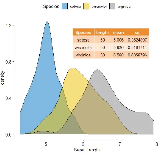
混合图
混合表、字体和图
# Density plot of "Sepal.Length"
#::::::::::::::::::::::::::::::::::::::
density.p <- ggdensity(iris, x = "Sepal.Length", fill = "Species", palette = "jco")
# Draw the summary table of Sepal.Length
#::::::::::::::::::::::::::::::::::::::
# Compute descriptive statistics by groups
stable <- desc_statby(iris, measure.var = "Sepal.Length",grps = "Species")
stable <- stable[, c("Species", "length", "mean", "sd")]
# Summary table plot, medium orange theme
stable.p <- ggtexttable(stable, rows = NULL, theme = ttheme("mOrange"))
# Draw text
#::::::::::::::::::::::::::::::::::::::
text <- paste("iris data set gives the measurements in cm","of the variables sepal length and width","and petal length and width, respectively,","for 50 flowers from each of 3 species of iris.","The species are Iris setosa, versicolor, and virginica.", sep = " ")
text.p <- ggparagraph(text = text, face = "italic", size = 11, color = "black")
# Arrange the plots on the same page
ggarrange(density.p, stable.p, text.p, ncol = 1, nrow = 3,heights = c(1, 0.5, 0.3))

-
注释table在图上
density.p <- ggdensity(iris, x = "Sepal.Length", fill = "Species", palette = "jco")
stable <- desc_statby(iris, measure.var = "Sepal.Length",grps = "Species")
stable <- stable[, c("Species", "length", "mean", "sd")]
stable.p <- ggtexttable(stable, rows = NULL, theme = ttheme("mOrange"))
density.p + annotation_custom(ggplotGrob(stable.p),xmin = 5.5, ymin = 0.7,xmax = 8)
systemic information
sessionInfo()
R version 3.6.1 (2019-07-05) Platform: x86_64-w64-mingw32/x64 (64-bit) Running under: Windows 10 x64 (build 19042) Matrix products: default locale: [1] LC_COLLATE=Chinese (Simplified)_China.936 LC_CTYPE=Chinese (Simplified)_China.936 [3] LC_MONETARY=Chinese (Simplified)_China.936 LC_NUMERIC=C [5] LC_TIME=Chinese (Simplified)_China.936 attached base packages: [1] stats graphics grDevices utils datasets methods base other attached packages: [1] ggpubr_0.4.0 ggplot2_3.3.2 loaded via a namespace (and not attached):[1] zip_2.0.4 Rcpp_1.0.3 cellranger_1.1.0 pillar_1.4.6 compiler_3.6.1 forcats_0.5.0 [7] tools_3.6.1 digest_0.6.27 lifecycle_0.2.0 tibble_3.0.4 gtable_0.3.0 pkgconfig_2.0.3 [13] rlang_0.4.8 openxlsx_4.2.3 ggsci_2.9 rstudioapi_0.10 curl_4.3 haven_2.3.1 [19] rio_0.5.16 withr_2.1.2 dplyr_1.0.2 generics_0.0.2 vctrs_0.3.4 hms_0.5.3 [25] grid_3.6.1 tidyselect_1.1.0 glue_1.4.2 data.table_1.13.2 R6_2.4.1 rstatix_0.6.0 [31] readxl_1.3.1 foreign_0.8-73 carData_3.0-4 farver_2.0.3 tidyr_1.0.0 purrr_0.3.3 [37] car_3.0-10 magrittr_1.5 scales_1.1.0 backports_1.1.10 ellipsis_0.3.1 abind_1.4-5 [43] colorspace_1.4-1 ggsignif_0.6.0 labeling_0.4.2 stringi_1.4.3 munsell_0.5.0 broom_0.7.2 [49] crayon_1.3.4
相关文章:
R可视化:ggpubr包学习
欢迎大家关注全网生信学习者系列: WX公zhong号:生信学习者 Xiao hong书:生信学习者 知hu:生信学习者 CDSN:生信学习者2 介绍 ggpubr是我经常会用到的R包,它傻瓜式的画图方式对很多初次接触R绘图的人来…...

优化Spring Boot项目启动时间:详解与实践
目录 引言了解Spring Boot框架启动机制常见启动瓶颈分析优化策略 禁用不必要的自动配置使用Profile进行开发和生产环境区分精简依赖延迟加载Bean并行初始化Bean缓存数据源连接优化Spring Data JPA使用Spring Boot DevTools 通过性能测试工具分析和优化实战示例:一个…...

Android如何简单快速实现RecycleView的拖动重排序功能
本文首发于公众号“AntDream”,欢迎微信搜索“AntDream”或扫描文章底部二维码关注,和我一起每天进步一点点 要实现这个拖动重排序功能,主要是用到了RecycleView的ItemTouchHelper类 首先是定义一个接口 interface ItemTouchHelperAdapter …...
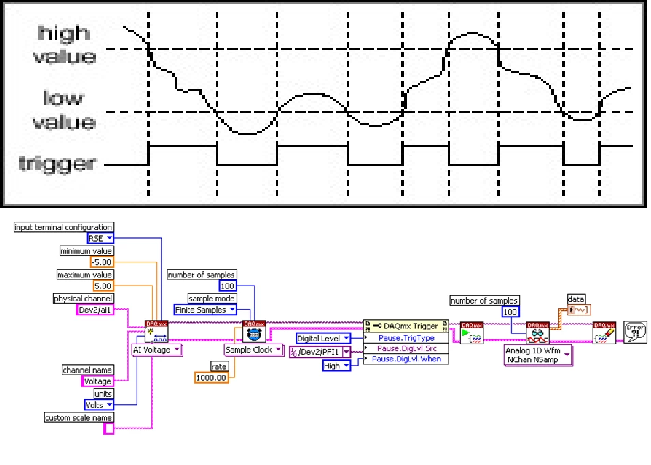
LabVIEW利用旋转编码器脉冲触发数据采集
利用旋转编码器发出的脉冲控制数据采集,可以采用硬件触发方式,以确保每个脉冲都能触发一次数据采集。本文提供了详细的解决方案,包括硬件连接、LabVIEW编程和触发设置,确保数据采集的准确性和实时性。 一、硬件连接 1. 旋转编码…...
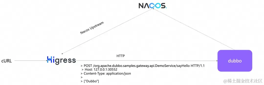
Dubbo3 服务原生支持 http 访问,兼具高性能与易用性
作者:刘军 作为一款 rpc 框架,Dubbo 的优势是后端服务的高性能的通信、面向接口的易用性,而它带来的弊端则是 rpc 接口的测试与前端流量接入成本较高,我们需要专门的工具或协议转换才能实现后端服务调用。这个现状在 Dubbo3 中得…...
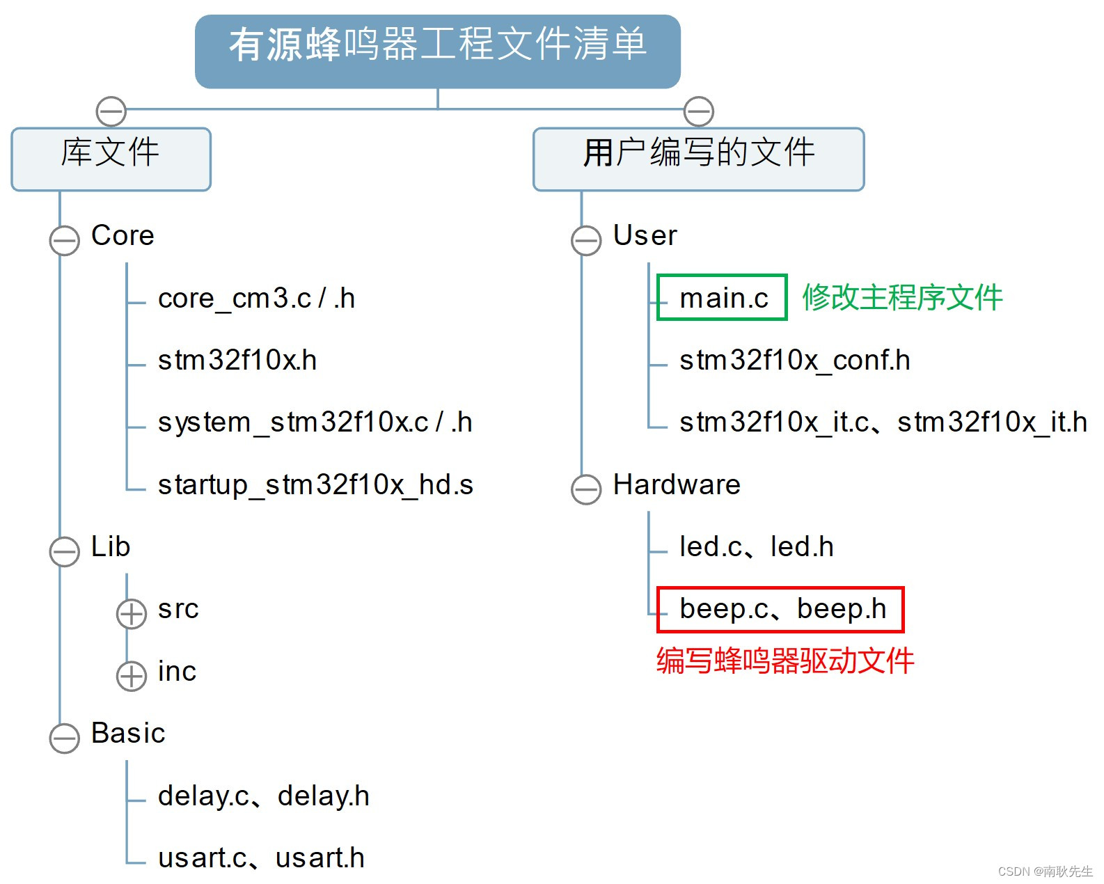
我在高职教STM32——GPIO入门之蜂鸣器
大家好,我是老耿,高职青椒一枚,一直从事单片机、嵌入式、物联网等课程的教学。对于高职的学生层次,同行应该都懂的,老师在课堂上教学几乎是没什么成就感的。正因如此,才有了借助 CSDN 平台寻求认同感和成就…...
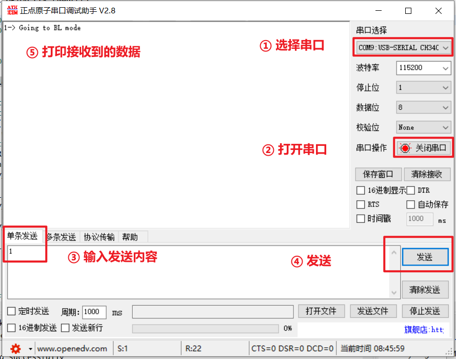
STM32 Customer BootLoader 刷新项目 (一) STM32CubeMX UART串口通信工程搭建
STM32 Customer BootLoader 刷新项目 (一) STM32CubeMX UART串口通信工程搭建 文章目录 STM32 Customer BootLoader 刷新项目 (一) STM32CubeMX UART串口通信工程搭建功能与作用典型工作流程 1. 硬件原理图介绍2. STM32 CubeMX工程搭建2.1 创建工程2.2 系统配置2.3 USART串口配…...

如果搜索一定超时,如何用dp来以空间换时间
E - Alphabet Tiles (atcoder.jp) 题目大意:1到k长度的字符串时,在A-Z给定数量下,搭配出多少种不同的字符串 思路 排列组合,会死人的 暴搜:可以解决,但是时间太长 dp:考虑前 i 个字母&…...

MySQL常见的命令
MySQL常见的命令 查看数据库(注意添加分号) show databases;进入到某个库 use 库; 例如:进入test use test;显示表格 show tables;直接展示某个库里面的表 show tables from 库; 例如:展示mysql中的表格 show tabl…...

11 类型泛化
11 类型泛化 1、函数模版1.1 前言1.2 函数模版1.3 隐式推断类型实参1.4 函数模板重载1.5 函数模板类型形参的默认类型(C11标准) 2、类模版2.1 类模板的成员函数延迟实例化2.2 类模板的静态成员2.3 类模板的递归实例化2.4 类模板类型形参缺省值 3、类模板…...
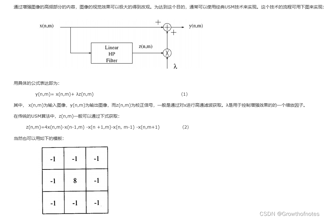
UE4_后期_ben_模糊和锐化滤镜
学习笔记,不喜勿喷,侵权立删,祝愿生活越来越好! 本篇教程主要介绍后期处理的简单模糊和锐化滤镜效果,学习之前首先要回顾下上节课介绍的屏幕扭曲效果: 这是全屏效果,然后又介绍了几种蒙版&#…...

Spring Boot中Excel的导入导出的实现之Apache POI框架使用教程
文章目录 前言一、Apache POI 是什么?二、使用 Apache POI 实现 Excel 的导入和导出① 导入 Excel1. 添加依赖2. 编写导入逻辑3. 在 Controller 中处理上传请求 ② 导出 Excel1. 添加依赖2. 编写导出逻辑3. 在 Controller 中处理导出请求 总结 前言 在 Spring Boot …...
CentOS搭建kubernetes集群详细过程(yum安装方式)
kubernetes集群搭建详细过程(yum安装方式) Kubernetes,也被称为K8s,是一个多功能的容器管理工具,它不仅能够协调和调度容器的部署,而且还能监控容器的健康状况并自动修复常见问题。这个平台是在谷歌十多年…...

Java 面试题:Java 的 Exception 和 Error 有什么区别?
在Java编程中,异常处理是确保程序稳健性和可靠性的重要机制。Java提供了一套完善的异常处理框架,通过捕获和处理异常,开发者可以有效地应对程序运行时可能出现的各种问题。在这一框架中,Exception和Error是两个核心概念࿰…...

在Vue 3中,el-select循环el-option的常见踩坑点,value值绑定对象类型?选中效果不准确?
在Vue 3中,el-select 组件是来自 Element Plus UI 库的一部分。 如果你想要设置默认选中的选项,你可以使用 v-model 来绑定选中的值。如果你想要在某个时刻让某个选项显示为已选中,可以设置对应的值到 v-model 绑定的数据。 <template>…...

Qt实现单例模式:Q_GLOBAL_STATIC和Q_GLOBAL_STATIC_WITH_ARGS
目录 1.引言 2.了解Q_GLOBAL_STATIC 3.了解Q_GLOBAL_STATIC_WITH_ARGS 4.实现原理 4.1.对象的创建 4.2.QGlobalStatic 4.3.宏定义实现 4.4.注意事项 5.总结 1.引言 设计模式之单例模式-CSDN博客 所谓的全局静态对象,大多是在单例类中所见,在之前…...
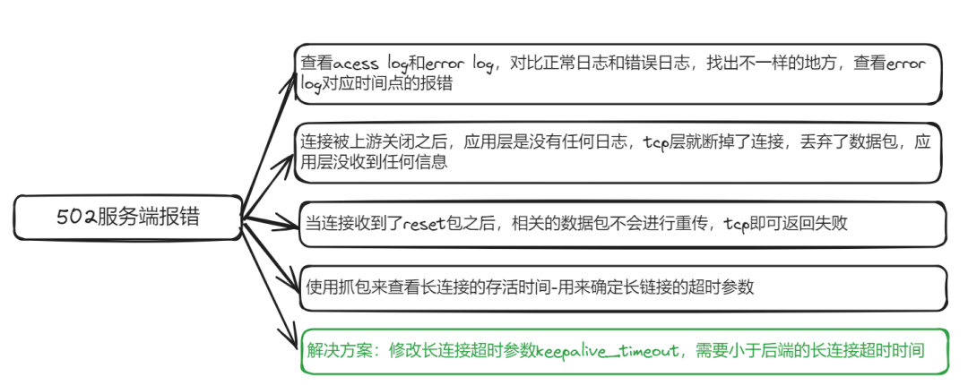
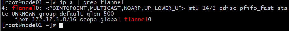
通过nginx转发后应用偶发502bad gateway
序言 学习了一些东西,如何才是真正自己能用的呢?好像就是看自己的潜意识的反应,例如解决了一个问题,那么下次再碰到类似的问题,能直接下意识的去找到对应的信息,从而解决,而不是和第一次碰到一样…...

linux中如何进行yum源的挂载
linux中如何进行yum源的挂载 1.首先创建目录[rootserver /]# mkdir /rhel92.使用mount命令进行、dev/cdrom/的镜像文件进行挂载[rootserver /]# mount /dev/cdrom /rhel9/ 注意:此时设立的是临时命令。重启后则失效,若想在下次开启后仍然挂载&a…...

ffmpeg的部署踩坑及简单使用方式
ffmpeg的使用方式有以下几种: 使用原生安装包 直接在ffmpeg官网上下载安装该软件,加入到环境变量中就可以使用了 优点:简单,灵活,代码中也不用添加其他第三方的包 缺点:需要手动安装ffmpeg,这点比较麻烦 部署-windows 在windows环境下,有时就算加入到了环境变量,…...
misc刷题记录2[陇剑杯 2021]
[陇剑杯 2021]webshell (1)单位网站被黑客挂马,请您从流量中分析出webshell,进行回答: 黑客登录系统使用的密码是_____________。得到的flag请使用NSSCTF{}格式提交。 这里我的思路是,既然要选择的时间段是黑客登录网站以后&…...

使用docker在3台服务器上搭建基于redis 6.x的一主两从三台均是哨兵模式
一、环境及版本说明 如果服务器已经安装了docker,则忽略此步骤,如果没有安装,则可以按照一下方式安装: 1. 在线安装(有互联网环境): 请看我这篇文章 传送阵>> 点我查看 2. 离线安装(内网环境):请看我这篇文章 传送阵>> 点我查看 说明:假设每台服务器已…...
《从零掌握MIPI CSI-2: 协议精解与FPGA摄像头开发实战》-- CSI-2 协议详细解析 (一)
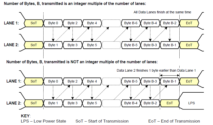
CSI-2 协议详细解析 (一) 1. CSI-2层定义(CSI-2 Layer Definitions) 分层结构 :CSI-2协议分为6层: 物理层(PHY Layer) : 定义电气特性、时钟机制和传输介质(导线&#…...

vue3 字体颜色设置的多种方式
在Vue 3中设置字体颜色可以通过多种方式实现,这取决于你是想在组件内部直接设置,还是在CSS/SCSS/LESS等样式文件中定义。以下是几种常见的方法: 1. 内联样式 你可以直接在模板中使用style绑定来设置字体颜色。 <template><div :s…...

Nuxt.js 中的路由配置详解
Nuxt.js 通过其内置的路由系统简化了应用的路由配置,使得开发者可以轻松地管理页面导航和 URL 结构。路由配置主要涉及页面组件的组织、动态路由的设置以及路由元信息的配置。 自动路由生成 Nuxt.js 会根据 pages 目录下的文件结构自动生成路由配置。每个文件都会对…...
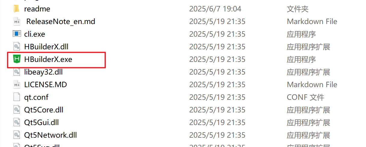
HBuilderX安装(uni-app和小程序开发)
下载HBuilderX 访问官方网站:https://www.dcloud.io/hbuilderx.html 根据您的操作系统选择合适版本: Windows版(推荐下载标准版) Windows系统安装步骤 运行安装程序: 双击下载的.exe安装文件 如果出现安全提示&…...

大学生职业发展与就业创业指导教学评价
这里是引用 作为软工2203/2204班的学生,我们非常感谢您在《大学生职业发展与就业创业指导》课程中的悉心教导。这门课程对我们即将面临实习和就业的工科学生来说至关重要,而您认真负责的教学态度,让课程的每一部分都充满了实用价值。 尤其让我…...

React---day11
14.4 react-redux第三方库 提供connect、thunk之类的函数 以获取一个banner数据为例子 store: 我们在使用异步的时候理应是要使用中间件的,但是configureStore 已经自动集成了 redux-thunk,注意action里面要返回函数 import { configureS…...

AI+无人机如何守护濒危物种?YOLOv8实现95%精准识别
【导读】 野生动物监测在理解和保护生态系统中发挥着至关重要的作用。然而,传统的野生动物观察方法往往耗时耗力、成本高昂且范围有限。无人机的出现为野生动物监测提供了有前景的替代方案,能够实现大范围覆盖并远程采集数据。尽管具备这些优势…...
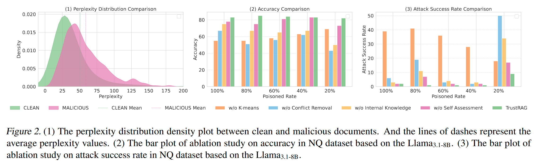
[论文阅读]TrustRAG: Enhancing Robustness and Trustworthiness in RAG
TrustRAG: Enhancing Robustness and Trustworthiness in RAG [2501.00879] TrustRAG: Enhancing Robustness and Trustworthiness in Retrieval-Augmented Generation 代码:HuichiZhou/TrustRAG: Code for "TrustRAG: Enhancing Robustness and Trustworthin…...

[USACO23FEB] Bakery S
题目描述 Bessie 开了一家面包店! 在她的面包店里,Bessie 有一个烤箱,可以在 t C t_C tC 的时间内生产一块饼干或在 t M t_M tM 单位时间内生产一块松糕。 ( 1 ≤ t C , t M ≤ 10 9 ) (1 \le t_C,t_M \le 10^9) (1≤tC,tM≤109)。由于空间…...