【人工智能】Python在机器学习与人工智能中的应用
Python因其简洁易用、丰富的库支持以及强大的社区,被广泛应用于机器学习与人工智能(AI)领域。本教程通过实用的代码示例和讲解,带你从零开始掌握Python在机器学习与人工智能中的基本用法。
1. 机器学习与AI的Python生态系统
Python拥有多种支持机器学习和AI的库,以下是几个核心库:
- NumPy:处理高效数组和矩阵运算。
- Pandas:提供数据操作与分析工具。
- Matplotlib/Seaborn:用于数据可视化。
- Scikit-learn:机器学习的核心库,包含分类、回归、聚类等算法。
- TensorFlow/PyTorch:深度学习框架,用于构建和训练神经网络。
安装:
pip install numpy pandas matplotlib scikit-learn tensorflow2. 数据预处理
加载数据
import pandas as pd# 示例数据
data = pd.DataFrame({'Feature1': [1, 2, 3, 4, 5],'Feature2': [5, 4, 3, 2, 1],'Target': [1, 0, 1, 0, 1]
})print(data)
输出:
   Feature1  Feature2  Target
0         1         5       1
1         2         4       0
2         3         3       1
3         4         2       0
4         5         1       1
特征缩放
归一化或标准化数据有助于提升模型性能。
import pandas as pd
from sklearn.preprocessing import MinMaxScalerdata = pd.DataFrame({'Feature1': [1, 2, 3, 4, 5],'Feature2': [5, 4, 3, 2, 1],'Target': [1, 0, 1, 0, 1]
})scaler = MinMaxScaler()
scaled_features = scaler.fit_transform(data[['Feature1', 'Feature2']])
print(scaled_features)
输出:
[[0. 1. ][0.25 0.75][0.5 0.5 ][0.75 0.25][1. 0. ]]3. 数据可视化
利用Matplotlib和Seaborn绘制数据分布图。
import pandas as pd
from sklearn.preprocessing import MinMaxScaler
import matplotlib.pyplot as plt
import seaborn as snsdata = pd.DataFrame({'Feature1': [1, 2, 3, 4, 5],'Feature2': [5, 4, 3, 2, 1],'Target': [1, 0, 1, 0, 1]
})scaler = MinMaxScaler()
scaled_features = scaler.fit_transform(data[['Feature1', 'Feature2']])
print(scaled_features)# 散点图
sns.scatterplot(x='Feature1', y='Feature2', hue='Target', data=data)
plt.title('Feature Scatter Plot')
plt.show()

4. 构建第一个机器学习模型
使用Scikit-learn实现分类模型。
拆分数据
import pandas as pd
from sklearn.model_selection import train_test_splitdata = pd.DataFrame({'Feature1': [1, 2, 3, 4, 5],'Feature2': [5, 4, 3, 2, 1],'Target': [1, 0, 1, 0, 1]
})X = data[['Feature1', 'Feature2']]
y = data['Target']X_train, X_test, y_train, y_test = train_test_split(X, y, test_size=0.2, random_state=42)print('X_train:')
print(X_train)
print('X_test:')
print(X_test)
print('y_train:')
print(y_train)
print('y_test:')
print(y_test)
X_train:Feature1  Feature2
4         5         1
2         3         3
0         1         5
3         4         2X_test:Feature1  Feature2
1         2         4y_train:
4    1
2    1
0    1
3    0
Name: Target, dtype: int64y_test:
1    0
Name: Target, dtype: int64
训练模型
import pandas as pd
from sklearn.model_selection import train_test_split
from sklearn.ensemble import RandomForestClassifier
from sklearn.metrics import accuracy_scoredata = pd.DataFrame({'Feature1': [1, 2, 3, 4, 5],'Feature2': [5, 4, 3, 2, 1],'Target': [1, 0, 1, 0, 1]
})X = data[['Feature1', 'Feature2']]
y = data['Target']X_train, X_test, y_train, y_test = train_test_split(X, y, test_size=0.2, random_state=42)# 随机森林分类器
model = RandomForestClassifier()
model.fit(X_train, y_train)# 预测
y_pred = model.predict(X_test)
print("Accuracy:", accuracy_score(y_test, y_pred))
Accuracy: 0.05. 深度学习与神经网络
构建一个简单的神经网络进行分类任务。
安装TensorFlow
conda install tensorflow如果安装遇到Could not solve for environment spec错误,请先执行以下命令
conda create -n tf_env python=3.8
conda activate tf_env
构建模型
import tensorflow as tf
from tensorflow.keras.models import Sequential
from tensorflow.keras.layers import Dense# 构建神经网络
model = Sequential([Dense(8, input_dim=2, activation='relu'),Dense(4, activation='relu'),Dense(1, activation='sigmoid')
])
编译与训练
model.compile(optimizer='adam', loss='binary_crossentropy', metrics=['accuracy'])
model.fit(X_train, y_train, epochs=50, batch_size=1, verbose=1)
评估模型
loss, accuracy = model.evaluate(X_test, y_test)
print("Loss:", loss)
print("Accuracy:", accuracy)
完整代码
import pandas as pd
from sklearn.model_selection import train_test_split
import tensorflow as tf
from tensorflow.keras.models import Sequential
from tensorflow.keras.layers import Densedata = pd.DataFrame({'Feature1': [1, 2, 3, 4, 5],'Feature2': [5, 4, 3, 2, 1],'Target': [1, 0, 1, 0, 1]
})X = data[['Feature1', 'Feature2']]
y = data['Target']X_train, X_test, y_train, y_test = train_test_split(X, y, test_size=0.2, random_state=42)# 构建神经网络
model = Sequential([Dense(8, input_dim=2, activation='relu'),Dense(4, activation='relu'),Dense(1, activation='sigmoid')
])model.compile(optimizer='adam', loss='binary_crossentropy', metrics=['accuracy'])
model.fit(X_train, y_train, epochs=50, batch_size=1, verbose=1)loss, accuracy = model.evaluate(X_test, y_test)
print("Loss:", loss)
print("Accuracy:", accuracy)
输出:
Epoch 1/50
4/4 [==============================] - 1s 1ms/step - loss: 0.6867 - accuracy: 0.5000
Epoch 2/50
4/4 [==============================] - 0s 997us/step - loss: 0.6493 - accuracy: 0.5000
Epoch 3/50
4/4 [==============================] - 0s 997us/step - loss: 0.6183 - accuracy: 0.5000
Epoch 4/50
4/4 [==============================] - 0s 665us/step - loss: 0.5920 - accuracy: 0.5000
Epoch 5/50
4/4 [==============================] - 0s 1ms/step - loss: 0.5702 - accuracy: 0.5000
Epoch 6/50
4/4 [==============================] - 0s 997us/step - loss: 0.5612 - accuracy: 0.7500
Epoch 7/50
4/4 [==============================] - 0s 998us/step - loss: 0.5405 - accuracy: 0.7500
Epoch 8/50
4/4 [==============================] - 0s 665us/step - loss: 0.5223 - accuracy: 0.7500
Epoch 9/50
4/4 [==============================] - 0s 1ms/step - loss: 0.5047 - accuracy: 0.7500
Epoch 10/50
4/4 [==============================] - 0s 665us/step - loss: 0.4971 - accuracy: 0.7500
Epoch 11/50
4/4 [==============================] - 0s 997us/step - loss: 0.4846 - accuracy: 0.7500
Epoch 12/50
4/4 [==============================] - 0s 997us/step - loss: 0.4762 - accuracy: 0.7500
Epoch 13/50
4/4 [==============================] - 0s 665us/step - loss: 0.4753 - accuracy: 0.7500
Epoch 14/50
4/4 [==============================] - 0s 997us/step - loss: 0.4623 - accuracy: 1.0000
Epoch 15/50
4/4 [==============================] - 0s 998us/step - loss: 0.4563 - accuracy: 1.0000
Epoch 16/50
4/4 [==============================] - 0s 998us/step - loss: 0.4530 - accuracy: 1.0000
Epoch 17/50
4/4 [==============================] - 0s 997us/step - loss: 0.4469 - accuracy: 1.0000
Epoch 18/50
4/4 [==============================] - 0s 997us/step - loss: 0.4446 - accuracy: 0.7500
Epoch 19/50
4/4 [==============================] - 0s 665us/step - loss: 0.4385 - accuracy: 0.7500
Epoch 20/50
4/4 [==============================] - 0s 998us/step - loss: 0.4355 - accuracy: 0.7500
Epoch 21/50
4/4 [==============================] - 0s 997us/step - loss: 0.4349 - accuracy: 0.7500
Epoch 22/50
4/4 [==============================] - 0s 665us/step - loss: 0.4290 - accuracy: 0.7500
Epoch 23/50
4/4 [==============================] - 0s 997us/step - loss: 0.4270 - accuracy: 0.7500
Epoch 24/50
4/4 [==============================] - 0s 997us/step - loss: 0.4250 - accuracy: 0.7500
Epoch 25/50
4/4 [==============================] - 0s 665us/step - loss: 0.4218 - accuracy: 0.7500
Epoch 26/50
4/4 [==============================] - 0s 997us/step - loss: 0.4192 - accuracy: 0.7500
Epoch 27/50
4/4 [==============================] - 0s 997us/step - loss: 0.4184 - accuracy: 0.7500
Epoch 28/50
4/4 [==============================] - 0s 665us/step - loss: 0.4152 - accuracy: 0.7500
Epoch 29/50
4/4 [==============================] - 0s 997us/step - loss: 0.4129 - accuracy: 0.7500
Epoch 30/50
4/4 [==============================] - 0s 997us/step - loss: 0.4111 - accuracy: 0.7500
Epoch 31/50
4/4 [==============================] - 0s 997us/step - loss: 0.4095 - accuracy: 0.7500
Epoch 32/50
4/4 [==============================] - 0s 997us/step - loss: 0.4070 - accuracy: 0.7500
Epoch 33/50
4/4 [==============================] - 0s 997us/step - loss: 0.4053 - accuracy: 0.7500
Epoch 34/50
4/4 [==============================] - 0s 997us/step - loss: 0.4033 - accuracy: 0.7500
Epoch 35/50
4/4 [==============================] - 0s 998us/step - loss: 0.4028 - accuracy: 0.7500
Epoch 36/50
4/4 [==============================] - 0s 997us/step - loss: 0.3998 - accuracy: 0.7500
Epoch 37/50
4/4 [==============================] - 0s 1ms/step - loss: 0.3978 - accuracy: 0.7500
Epoch 38/50
4/4 [==============================] - 0s 997us/step - loss: 0.3966 - accuracy: 0.7500
Epoch 39/50
4/4 [==============================] - 0s 665us/step - loss: 0.3946 - accuracy: 0.7500
Epoch 40/50
4/4 [==============================] - 0s 997us/step - loss: 0.3926 - accuracy: 0.7500
Epoch 41/50
4/4 [==============================] - 0s 997us/step - loss: 0.3918 - accuracy: 0.7500
Epoch 42/50
4/4 [==============================] - 0s 997us/step - loss: 0.3898 - accuracy: 0.7500
Epoch 43/50
4/4 [==============================] - 0s 997us/step - loss: 0.3877 - accuracy: 0.7500
Epoch 44/50
4/4 [==============================] - 0s 997us/step - loss: 0.3861 - accuracy: 0.7500
Epoch 45/50
4/4 [==============================] - 0s 665us/step - loss: 0.3842 - accuracy: 0.7500
Epoch 46/50
4/4 [==============================] - 0s 665us/step - loss: 0.3830 - accuracy: 0.7500
Epoch 47/50
4/4 [==============================] - 0s 997us/step - loss: 0.3815 - accuracy: 0.7500
Epoch 48/50
4/4 [==============================] - 0s 665us/step - loss: 0.3790 - accuracy: 0.7500
Epoch 49/50
4/4 [==============================] - 0s 665us/step - loss: 0.3778 - accuracy: 0.7500
Epoch 50/50
4/4 [==============================] - 0s 997us/step - loss: 0.3768 - accuracy: 0.7500
1/1 [==============================] - 0s 277ms/step - loss: 2.8638 - accuracy: 0.0000e+00
Loss: 2.863826274871826
Accuracy: 0.0
6. 数据聚类
实现一个K-Means聚类模型:
from sklearn.cluster import KMeans# 数据
data_points = [[1, 2], [2, 3], [3, 4], [8, 7], [9, 8], [10, 9]]# K-Means
kmeans = KMeans(n_clusters=2)
kmeans.fit(data_points)# 输出聚类中心
print("Cluster Centers:", kmeans.cluster_centers_)
输出:
Cluster Centers: [[9. 8.][2. 3.]]7. 自然语言处理 (NLP)
使用NLTK处理文本数据:
pip install nltk文本分词
import nltknltk.download('punkt_tab')
nltk.download('punkt')from nltk.tokenize import word_tokenizetext = "Machine learning is amazing!"
tokens = word_tokenize(text)
print(tokens)
输出:
['Machine', 'learning', 'is', 'amazing', '!']词袋模型
from sklearn.feature_extraction.text import CountVectorizertexts = ["I love Python", "Python is great for AI"]
vectorizer = CountVectorizer()
X = vectorizer.fit_transform(texts)print(X.toarray())
输出:
[[0 0 0 0 1 1][1 1 1 1 0 1]]8. 实用案例:房价预测
from sklearn.datasets import fetch_california_housing
from sklearn.model_selection import train_test_split
from sklearn.linear_model import LinearRegression
from sklearn.metrics import mean_squared_error# 加载数据集
data = fetch_california_housing(as_frame=True)
X = data.data
y = data.target# 数据拆分
X_train, X_test, y_train, y_test = train_test_split(X, y, test_size=0.2, random_state=42)# 模型训练
model = LinearRegression()
model.fit(X_train, y_train)# 预测
y_pred = model.predict(X_test)
print("Model Coefficients:", model.coef_)# 评估
mse = mean_squared_error(y_test, y_pred)
print(f"Mean Squared Error: {mse}")
输出:
Model Coefficients: [ 4.48674910e-01  9.72425752e-03 -1.23323343e-01  7.83144907e-01-2.02962058e-06 -3.52631849e-03 -4.19792487e-01 -4.33708065e-01]
Mean Squared Error: 0.5558915986952442
总结
本教程涵盖了Python在机器学习和人工智能领域的基础应用,从数据预处理、可视化到模型构建和评估,再到深度学习的基本实现。通过这些示例,你可以逐步掌握如何使用Python进行机器学习和AI项目开发。
相关文章:
【人工智能】Python在机器学习与人工智能中的应用
Python因其简洁易用、丰富的库支持以及强大的社区,被广泛应用于机器学习与人工智能(AI)领域。本教程通过实用的代码示例和讲解,带你从零开始掌握Python在机器学习与人工智能中的基本用法。 1. 机器学习与AI的Python生态系统 Pyth…...

使用八爪鱼爬虫抓取汽车网站数据,分析舆情数据
我是做汽车行业的,可以用八爪鱼爬虫抓取汽车之家和微博上的汽车文章内容,分析各种电动汽车口碑数据。 之前,我写过很多Python网络爬虫的案例,使用requests、selenium等技术采集数据,这次尝试去采集小米SU7在微博、汽车…...

什么是事务?事务有哪些特性?
在数据库管理中,事务是一个核心概念,它确保了数据操作的完整性和一致性。本文将探讨事务的定义及其四大特性。 一、事务的定义 事务是数据库操作的最小工作单元,是作为单个逻辑工作单元执行的一系列操作。这些操作作为一个整体一起向系统提…...
)
玩转合宙Luat教程 基础篇④——程序基础(库、线程、定时器和订阅/发布)
文章目录 一、前言二、库三、线程四、定时器五、订阅/发布5.1 回调函数5.2 堵塞等待一、前言 教程目录大纲请查阅:玩转合宙Luat教程——导读 写一写Lua程序基础的东西。 包括如何调用库,如何创建线程、如何创建定时器,如何使用订阅/发布事件。 二、库 程序从main.lua开始通…...

24.<Spring博客系统①(数据库+公共代码+持久层+显示博客列表+博客详情)>
项目整体预览 登录页面 主页 查看全文 编辑 写博客 PS:Service.impl(现在流行写法) 推荐写法。后续完成项目。会尝试这样写。 接口可以有多个实现。每个实现都可以不同。 这也算一种设计模式。叫做(策略模式)。 我们…...
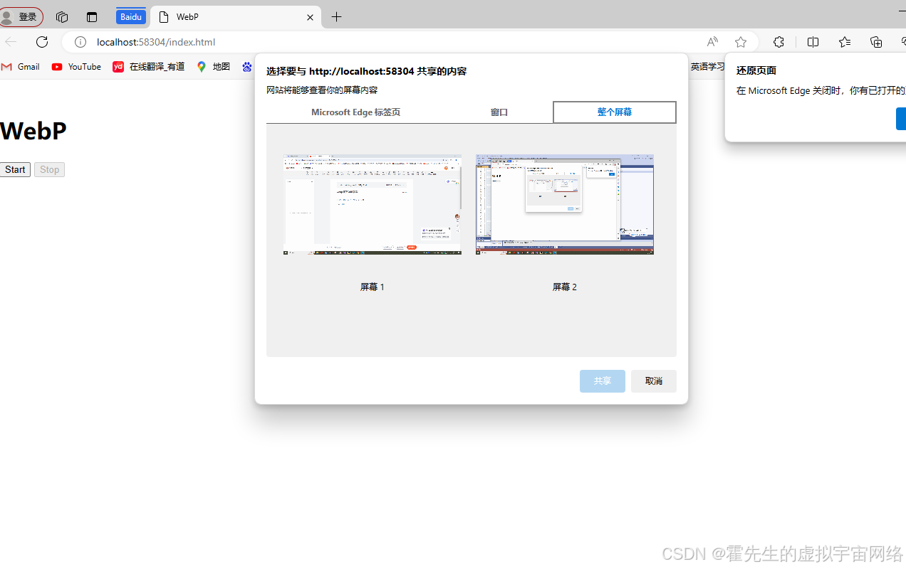
webp 网页如何录屏?
工作中正好研究到了一点:记录下这里: 先看下效果: 具体实现代码:  <!DOCTYPE html> <html lang"zh-CN"> <head><meta charset"UTF-8"><meta name"viewport&qu…...

丹摩征文活动|实现Llama3.1大模型的本地部署
文章目录 1.前言2.丹摩的配置3.Llama3.1的本地配置4. 最终界面 丹摩 1.前言 Llama3.1是Meta 公司发布的最新开源大型语言模型,相较于之前的版本,它在规模和功能上实现了显著提升,尤其是最大的 4050亿参数版本,成为开源社区中非常…...

Spring Boot 2 和 Spring Boot 3 中使用 Spring Security 的区别
文章目录 Spring Boot 2 和 Spring Boot 3 中使用 Spring Security 的区别1. Jakarta EE 迁移2. Spring Security 配置方式的变化3. PasswordEncoder 加密方式的变化4. permitAll() 和 authenticated() 的变化5. 更强的默认安全设置6. Java 17 支持与语法提升7. PreAuthorize、…...

【数据结构与算法】 LeetCode:回溯
文章目录 回溯算法组合组合总和(Hot 100)组合总和 II电话号码的字母组合(Hot 100)括号生成(Hot 100)分割回文串(Hot 100)复原IP地址子集(Hot 100)全排列&…...

SpringBoot线程池的使用
SpringBoot线程池的使用 在现代Web应用开发中,特别是在使用Spring Boot框架时,合理使用线程池可以显著提高应用的性能和响应速度。线程池不仅能够减少线程创建和销毁的开销,还能有效地控制并发任务的数量,避免因线程过多而导致的…...
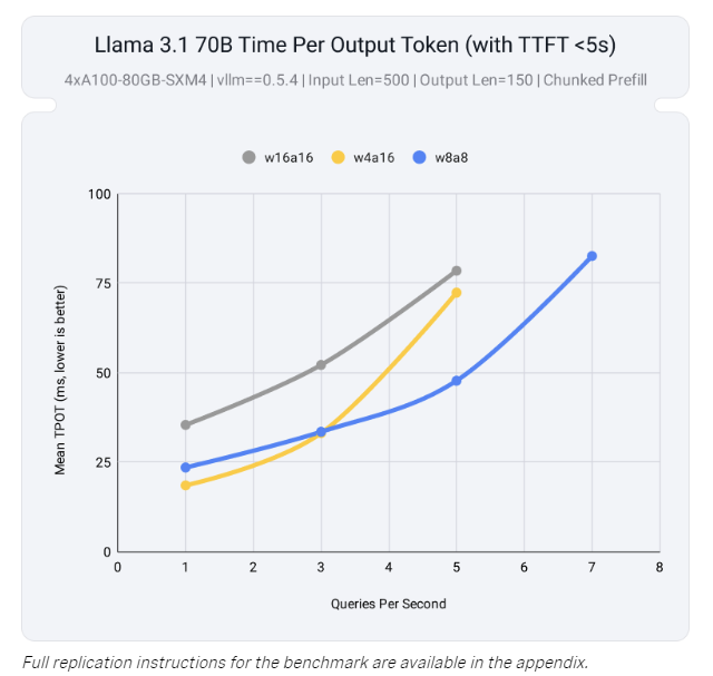
Neural Magic 发布 LLM Compressor:提升大模型推理效率的新工具
每周跟踪AI热点新闻动向和震撼发展 想要探索生成式人工智能的前沿进展吗?订阅我们的简报,深入解析最新的技术突破、实际应用案例和未来的趋势。与全球数同行一同,从行业内部的深度分析和实用指南中受益。不要错过这个机会,成为AI领…...

HttpServletRequest req和前端的关系,req.getParameter详细解释,req.getParameter和前端的关系
HttpServletRequest 对象在后端和前端之间起到了桥梁的作用,它包含了来自客户端的所有请求信息。通过 HttpServletRequest 对象,后端可以获取前端发送的请求参数、请求头、请求方法等信息,并根据这些信息进行相应的处理。以下是对 HttpServle…...

React-useEffect的使用
useEffect react提供的一个常用hook,用于在函数组件中执行副作用操作,比如数据获取、订阅或手动更改DOM。 基本用法: 接受2个参数: 一个包含命令式代码的函数(副作用函数)。一个依赖项数组,用…...

MySQL数据库与Informix:能否创建同名表?
MySQL数据库与Informix:能否创建同名表? 一、MySQL数据库中的同名表创建1. 使用CREATE TABLE ... SELECT语句2. 使用CREATE TABLE LIKE语句3. 复制表结构并选择性复制数据4. 使用同义词(Synonym)二、Informix数据库中的同名表创建1. 使用不同所有者2. 使用不同模式3. 复制表…...

爬虫实战:采集知乎XXX话题数据
目录 反爬虫的本意和其带来的挑战目标实战开发准备代码开发发现问题1. 发现问题[01]2. 发现问题[02] 解决问题1. 解决问题[01]2. 解决问题[02] 最终结果 结语 反爬虫的本意和其带来的挑战 在这个数字化时代社交媒体已经成为人们表达观点的重要渠道,对企业来说&…...

大数据新视界 -- Hive 数据桶原理:均匀分布数据的智慧(上)(9/ 30)
💖💖💖亲爱的朋友们,热烈欢迎你们来到 青云交的博客!能与你们在此邂逅,我满心欢喜,深感无比荣幸。在这个瞬息万变的时代,我们每个人都在苦苦追寻一处能让心灵安然栖息的港湾。而 我的…...

【小白学机器学习33】 大数定律python的 pandas.Dataframe 和 pandas.Series基础内容
目录 0 总结 0.1pd.Dataframe有一个比较麻烦琐碎的地方,就是引号 和括号 0.2 pd.Dataframe关于括号的原则 0.3 分清楚几个数据类型和对应的方法的范围 0.4 几个数据结构的构造关系 list → np.array(list) → pd.Series(np.array)/pd.Dataframe 1 python 里…...

【shodan】(五)网段利用
shodan基础(五) 声明:该笔记为up主 泷羽的课程笔记,本节链接指路。 警告:本教程仅作学习用途,若有用于非法行为的,概不负责。 nsa ip address range www.nsa.gov需科学上网 搜索网段 shodan s…...
)
LeetCode739. 每日温度(2024冬季每日一题 15)
给定一个整数数组 temperatures ,表示每天的温度,返回一个数组 answer ,其中 answer[i] 是指对于第 i 天,下一个更高温度出现在几天后。如果气温在这之后都不会升高,请在该位置用 0 来代替。 示例 1: 输入: temperatu…...

Node.js的http模块:创建HTTP服务器、客户端示例
新书速览|Vue.jsNode.js全栈开发实战-CSDN博客 《Vue.jsNode.js全栈开发实战(第2版)(Web前端技术丛书)》(王金柱)【摘要 书评 试读】- 京东图书 (jd.com) 要使用http模块,只需要在文件中通过require(http)引入即可。…...

终极指南:5步掌握GLM-4-Voice智能语音对话系统
终极指南:5步掌握GLM-4-Voice智能语音对话系统 【免费下载链接】GLM-4-Voice GLM-4-Voice | 端到端中英语音对话模型 项目地址: https://gitcode.com/gh_mirrors/gl/GLM-4-Voice 想要构建真正智能的语音对话AI吗?GLM-4-Voice作为智谱AI推出的端到…...

别再只盯着Mesh了!聊聊NoC拓扑选型:从Ring、Torus到Fat Tree,你的芯片设计该怎么选?
芯片设计中的NoC拓扑选型实战指南:从Ring到Fat Tree的深度权衡 当你在设计一款高性能芯片时,是否曾为选择合适的片上网络(NoC)拓扑而纠结?面对Ring、Mesh、Torus、Fat Tree等多种选项,每个决策都可能直接影响芯片的性能、功耗和面…...
)
告别AppImage:在Ubuntu上源码编译QGroundControl地面站(QT项目实战)
从源码构建QGroundControl:Ubuntu开发者深度指南 为什么选择源码编译而非AppImage? 在无人机开发领域,QGroundControl(QGC)作为PX4生态的核心地面站软件,其预编译的AppImage包虽然提供了开箱即用的便利性&a…...

网络安全人才平均年薪 24.09 万,跳槽周期 31 个月,安全工程师现状大曝光!
网络安全作为近两年兴起的热门行业,成了很多就业无门但是想转行的人心中比较向往但是又心存疑惑的行业,毕竟网络安全的发展史比较短,而国内目前网安的环境和市场情况还不算为大众所知晓,所以到底零基础转行入门网络安全之后&#…...
)
IEEE论文必备:LaTeX伪代码排版全攻略(附algorithmic与algorithm2e对比)
IEEE论文伪代码排版实战指南:从algorithmic到algorithm2e的深度解析 第一次在IEEE论文里插入伪代码时,我盯着编译报错发了半小时呆——明明本地预览完美无缺,上传到Overleaf却显示"undefined control sequence"。后来才发现是忘了在…...

商业逻辑和产品本质的庖丁解牛
“商业逻辑”与“产品本质”,常被混淆为“怎么赚钱”和“功能列表”。 但本质上: 商业逻辑是价值交换的闭环:谁为谁解决了什么问题,谁为此付费,利润从何而来,如何持续。产品本质是需求的具象化解决方案&…...

构建企业级知识库语义搜索引擎:NLP-StructBERT与MySQL协同实战
构建企业级知识库语义搜索引擎:NLP-StructBERT与MySQL协同实战 你是不是也遇到过这样的烦恼?公司内部堆积如山的文档、报告、产品手册,当你想找一份关于“如何解决客户退款流程中的常见问题”的资料时,在搜索框里输入“退款 流程…...

“Token”有了中文名:词元
作者|周雅3月23日,在中国发展高层论坛2026年年会上,国家数据局局长刘烈宏正式给出Token 的中文名——「词元」。如果只把这件事理解为一次术语翻译,可能会低估它。更值得注意的是,刘烈宏同时给了「词元」一个更明确的产…...
)
别再手动抄表了!用Python+Snap7实时采集S7-1200数据到Excel(附完整代码)
工业自动化数据采集实战:PythonSnap7实现S7-1200实时数据归档系统 在智能制造和工业4.0的浪潮中,生产设备的实时数据采集已成为工厂数字化升级的基础环节。传统的手动抄表方式不仅效率低下,还容易引入人为误差。本文将展示如何构建一个基于P…...

C语言完美演绎5-6
/* 范例:5-6 */#include <stdio.h>void main(void){int a;a2; /* 将整数2赋予给变量a,变量a的类型与整数2一样*/printf("a%d\n",a);a6.83; /* 将浮点数6.83重新赋予给变量a,浮点数6.83可以自动转型为int并赋予给变量a …...