荟萃分析R Meta-Analyses 3 Effect Sizes
总结
-
效应量是荟萃分析的基石。为了进行荟萃分析,我们至少需要估计效应大小及其标准误差。
-
效应大小的标准误差代表研究对效应估计的精确程度。荟萃分析以更高的精度和更高的权重给出效应量,因为它们可以更好地估计真实效应。
-
我们可以在荟萃分析中使用多种效应大小。常见的是“单变量”关系度量(例如平均值和比例)、相关性、(标准化)均值差以及风险、优势和发生率比率。
-
效应大小也可能存在偏差,例如由于测量误差和范围限制。有一些公式可以纠正一些偏差,包括标准化均值差异的小样本偏差、由于不可靠性导致的衰减以及范围限制问题。
-
其他常见问题是研究报告以不同格式计算效应量所需的数据,以及分析单位问题,当研究贡献不止一种效应量时就会出现这种问题
在第1.1章中,我们将荟萃分析定义为一种总结多项研究定量结果的技术。在荟萃分析中,研究而不是个人成为我们分析的基本单位。
这带来了新的问题。在初步研究中,通常很容易计算汇总统计数据,通过它我们可以描述我们收集的数据。例如,在初步研究中,通常计算连续结果的算术平均值 \(\bar{x}\)和标准差 \(s\) 。
然而,这是可能的,因为在初步研究中通常满足一个基本先决条件:我们知道所有研究对象的结果变量都是以相同的方式测量的。对于荟萃分析,通常不满足此假设。想象一下,我们想要进行一项荟萃分析,我们感兴趣的结果是八年级学生的数学技能。即使我们应用严格的纳入标准(参见第1.4.1章),也可能并非每项研究都使用完全相同的测试来衡量数学技能;有些甚至可能只报告通过或未通过测试的学生比例。这使得几乎不可能直接定量合成结果。
为了进行荟萃分析,我们必须找到一个可以总结所有研究的效应大小。有时,这样的效应量可以直接从出版物中提取;更多时候,我们必须根据研究中报告的其他数据来计算它们。所选的效应量指标可能会对荟萃分析的结果及其可解释性产生重大影响。因此,它们应该满足一些重要标准(Lipsey 和 Wilson 2001;Julian Higgins 等人 2019)。特别是,为荟萃分析选择的效应量测量应该是:
Comparable. It is important that the effect size measure has the same meaning across all studies. Let us take math skills as an example again. It makes no sense to pool differences between experimental and control groups in the number of points achieved on a math test when studies used different tests. Tests may, for example, vary in their level of difficulty, or in the maximum number of points that can be achieved.
Computable. We can only use an effect size metric for our meta-analysis if it is possible to derive its numerical value from the primary study. It must be possible to calculate the effect size for all of the included studies based on their data.
Reliable. Even if it is possible to calculate an effect size for all included studies, we must also be able to pool them statistically. To use some metric in meta-analyses, it must be at least possible to calculate the standard error (see next chapter). It is also important that the format of the effect size is suited for the meta-analytic technique we want to apply, and does not lead to errors or biases in our estimate.
Interpretable. The type of effect size we choose should be appropriate to answer our research question. For example, if we are interested in the strength of an association between two continuous variables, it is conventional to use correlations to express the size of the effect. It is relatively straightforward to interpret the magnitude of a correlation, and many researchers can understand them. In the following chapters, we will learn that it is sometimes not possible to use outcome measures which are both easy to interpret and ideal for our statistical computations. In such cases, it is necessary to transform effect sizes to a format with better mathematical properties before we pool them.
It is very likely that you have already stumbled upon the term “effect size” before. We also used the word here, without paying too much attention to what it precisely stands for. In the next section, we should therefore explore what we actually mean when we talk about an “effect size”.

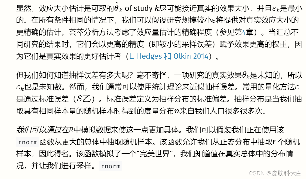
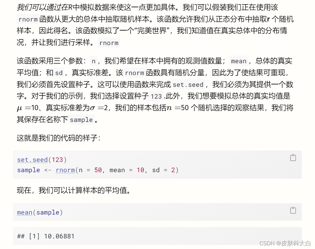
我们看到平均值是 ̄X==10.07,这已经非常接近我们人口的真实值。现在可以通过重复我们在这里所做的事情(随机抽样并计算其平均值)无数次来创建抽样分布。为了为您模拟这个过程,我们执行了之前的步骤 1000 次。
图3.1中的直方图显示了结果。我们可以看到样本的均值非常类似于均值为 10 的正态分布。如果我们抽取更多样本,均值的分布将更加接近正态分布。这一想法在统计学最基本的原则之一——中心极限定理中得到了表达 (Aronow 和 Miller 2019,第 3.2.4 章)。
。
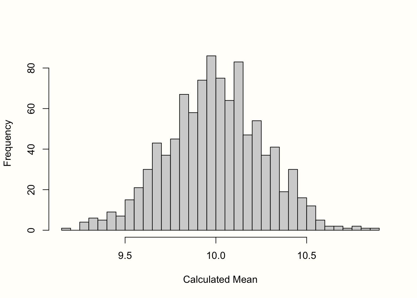
图 3.1:均值的“抽样分布”(1000 个样本)。
标准误差定义为该抽样分布的标准偏差。因此,我们计算了 1000 个模拟均值的标准差,以获得标准误差的近似值。结果是S乙=�乙=0.267。
正如我们之前提到的,我们不能简单地通过模拟真实的抽样分布来计算现实生活中的标准误差。然而,有一些基于统计理论的公式可以让我们计算标准误差的估计值,即使我们仅限于一个观察到的样本(通常是这样)。计算平均值标准误差的公式定义如下: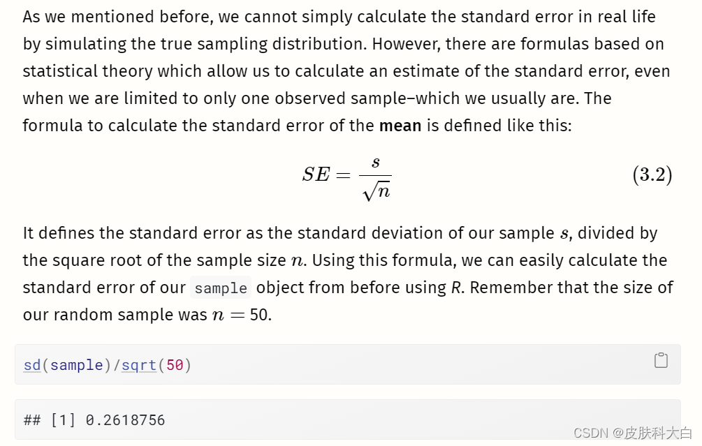

如果我们将该值与我们在抽样分布模拟中发现的值进行比较,我们会发现它们几乎相同。使用该公式,我们可以仅使用我们手头的样本来相当准确地估计标准误差。
在公式 3.2 中,我们可以看到平均值的标准误差取决于研究的样本量。什么时候n�变大,标准误差变小,这意味着研究对真实总体平均值的估计变得更加精确。
为了举例说明这种关系,我们进行了另一次模拟。我们再次使用该rnorm函数,并假设真实总体平均值为μ=�=10 以及那个σ=�=2.但这一次,我们改变了样本量,从n=�=2 至n=�=500. 对于每次模拟,我们使用公式 3.2 计算平均值和标准误差。
## Warning: Using `size` aesthetic for lines was deprecated in ggplot2
## 3.4.0.
## ℹ Please use `linewidth` instead.
## This warning is displayed once every 8 hours.
## Call `lifecycle::last_lifecycle_warnings()` to see where this
## warning was generated.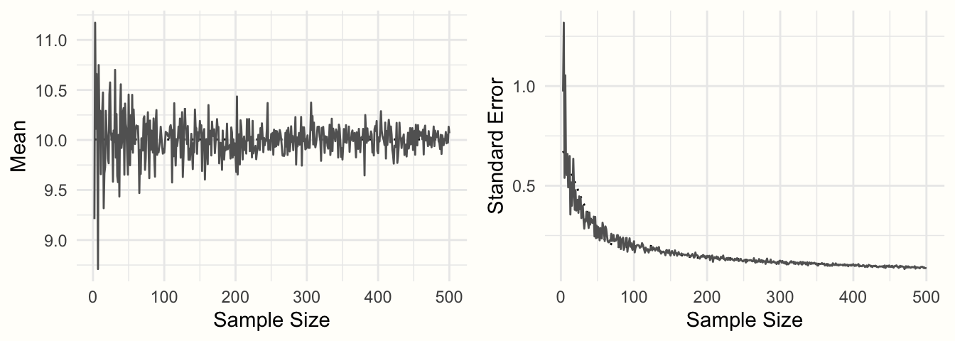
图 3.2:样本平均值和标准误差与样本量的函数关系。
图3.2显示了结果。我们可以看到均值看起来像一个漏斗:随着样本量的增加,均值估计变得越来越精确,并向 10 收敛。这种精度的增加由标准误差表示:随着样本量的增加,标准误差变得越来越小。
我们现在已经探索了进行荟萃分析所需的典型要素:(1)观察到的效应大小或结果测量,以及(2)其精度,以标准误差表示。如果这两类信息可以从已发表的研究中计算出来,通常也可以进行元分析综合(参见第4章)。
在我们的模拟中,我们使用变量的平均值作为示例。重要的是要理解,我们在上面看到的属性也可以在其他结果度量中找到,包括常用的效应量。如果我们计算样本中的平均差而不是平均值,则该平均差将表现出类似形状的抽样分布,并且平均差的标准误差也会随着样本量的增加而减小(假设标准差为保持不变)。同样的情况也成立,例如,(Fisher 的z�变换)相关性。
在以下部分中,我们将介绍荟萃分析中最常用的效应大小和结果测量。这些效应大小指标被如此频繁使用的一个原因是它们满足我们在本章开头定义的两个标准:它们是可靠的和可计算的。
在公式 3.2 中,我们描述了如何计算平均值的标准误差,但该公式只能轻松应用于平均值。其他效应大小和结果测量需要不同的公式来计算标准误差。对于我们在这里介绍的效应大小指标,幸运的是这些公式存在,我们将向您展示所有这些公式。公式的集合也可以在附录中找到。其中一些公式有些复杂,但好消息是我们几乎不需要手动计算标准误差。R中有多种函数可以为我们完成繁重的工作。
在下一节中,我们不仅想提供不同效应大小指标的理论讨论。我们还向您展示了您必须在数据集中准备哪些类型的信息,以便我们稍后使用的R荟萃分析函数可以轻松地为我们计算效应大小。
我们根据效应大小通常出现的研究设计类型对效应大小进行分组:观察设计(例如自然研究或调查)和实验设计(例如对照临床试验)。请注意,这只是一个粗略的分类,而不是严格的规则。我们提出的许多效应量在技术上适用于任何类型的研究设计,只要结果数据的类型适合。

# Set seed of 123 for reproducibility
# and take a random sample (n=50).
set.seed(123)
sample <- rnorm(n = 50, mean = 20, sd = 5)# Calculate the mean
mean(sample)
## [1] 20.17202# Calculate the standard error
sd(sample)/sqrt(50)## [1] 0.6546889为了进行均值荟萃分析,我们的数据集至少应包含以下列:
n。研究中的观察次数(样本量)。mean。研究中报告的平均值。sd。研究中报告的变量的标准差。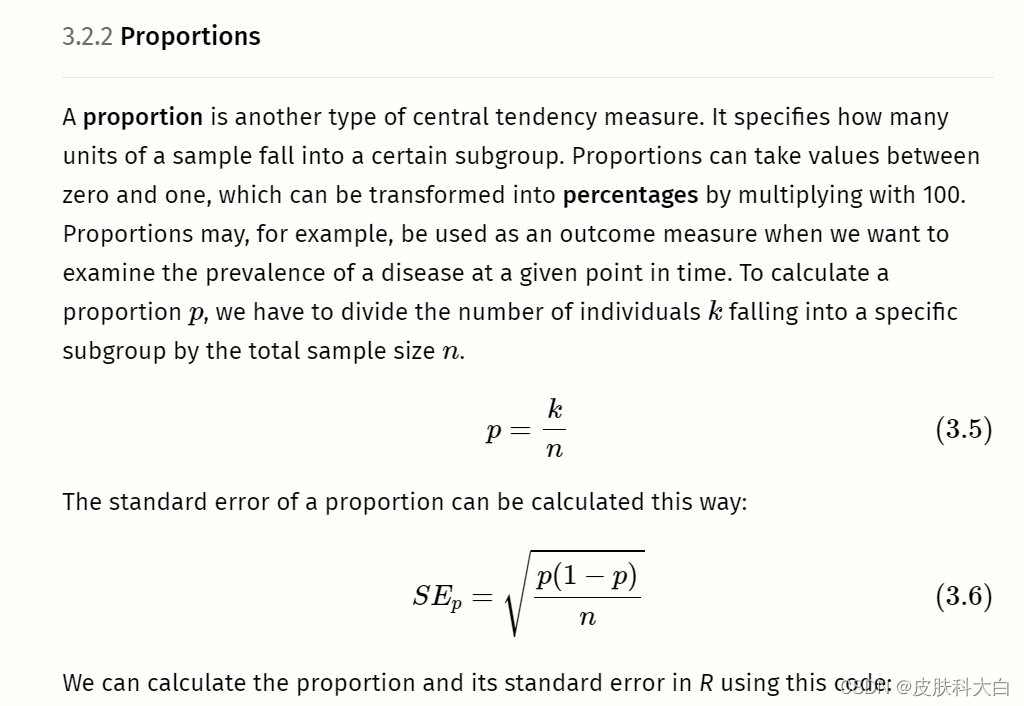
# We define the following values for k and n:
k <- 25
n <- 125# Calculate the proportion
p <- k/n
p
## [1] 0.2# Calculate the standard error
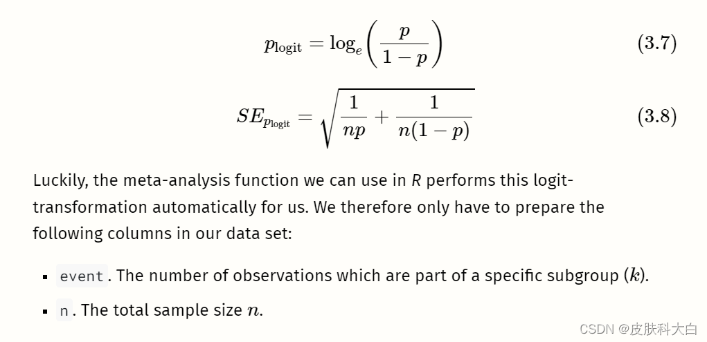
sqrt((p*(1-p))/n)## [1] 0.03577709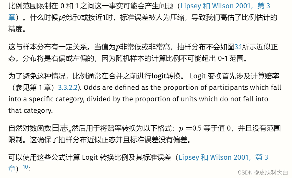


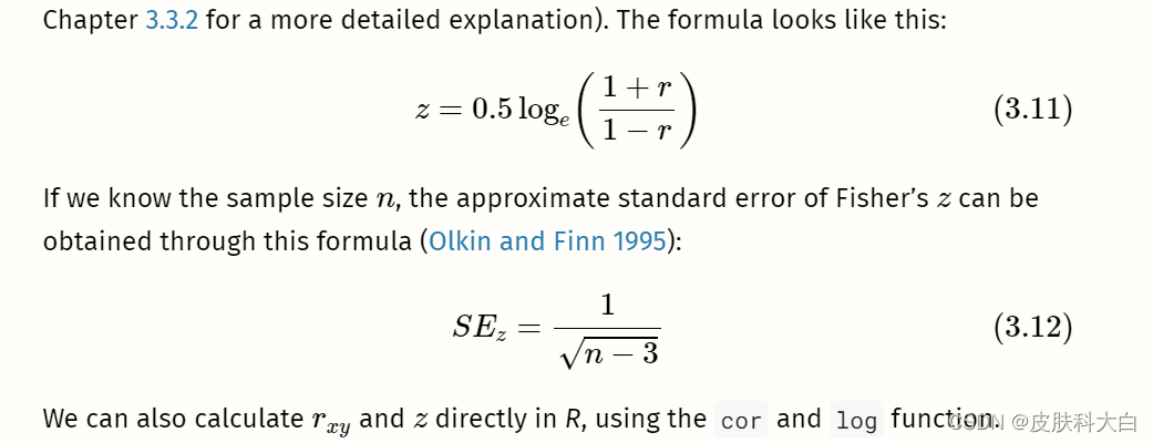
# Simulate two continuous variables x and y
set.seed(12345)
x <- rnorm(20, 50, 10)
y <- rnorm(20, 10, 3)# Calculate the correlation between x and y
r <- cor(x,y)
r
# Calculate Fisher's z
z <- 0.5*log((1+r)/(1-r))
z


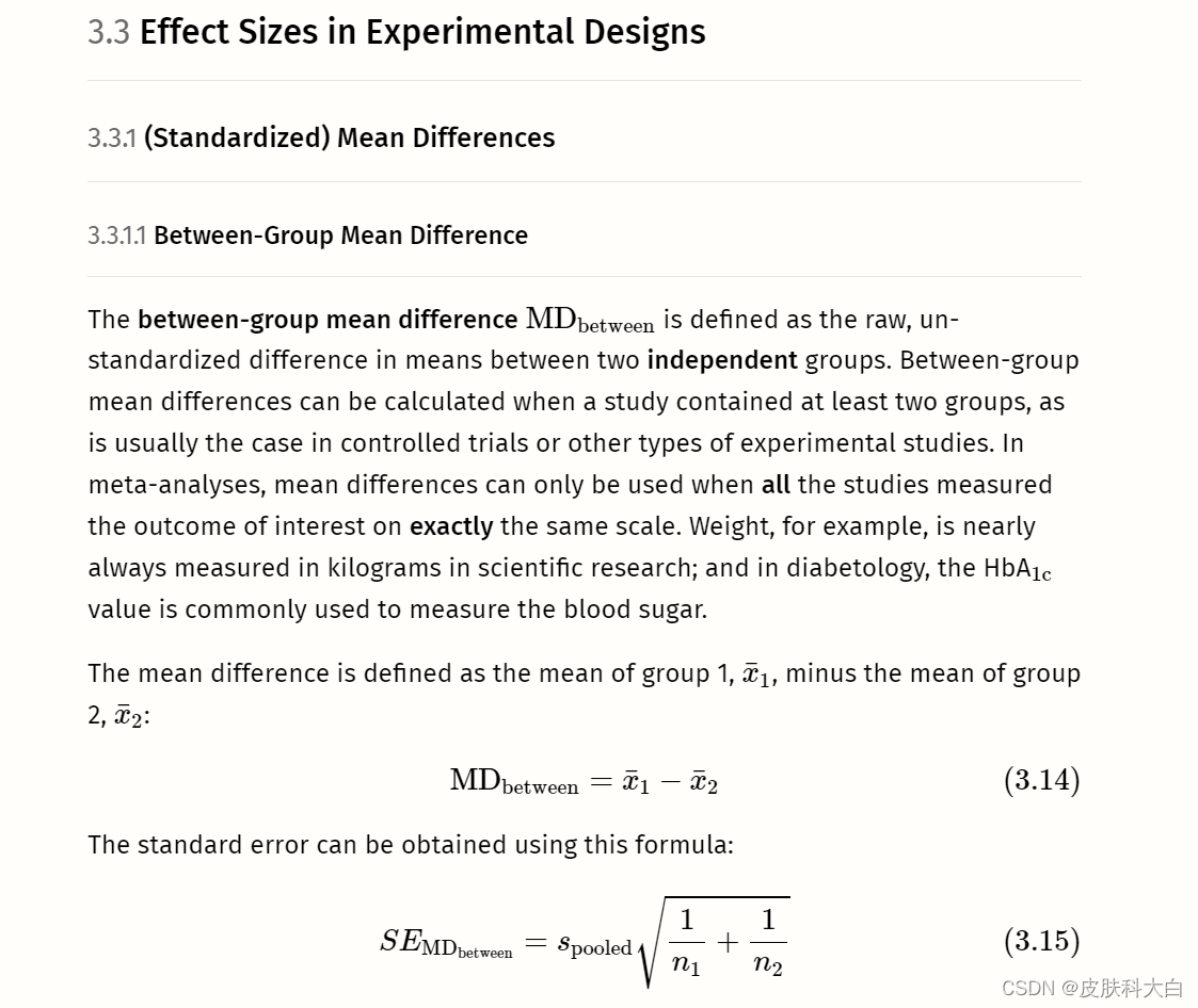
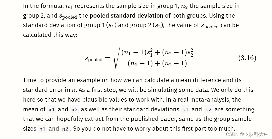
# Generate two random variables with different population means
set.seed(123)
x1 <- rnorm(n = 20, mean = 10, sd = 3)
x2 <- rnorm(n = 20, mean = 15, sd = 3)# Calculate values we need for the formulas
s1 <- sd(x1)
s2 <- sd(x2)
n1 <- 20
n2 <- 20
With this data at hand, we can proceed to the core part, in which we calculate the mean difference and its standard error using the formulae we showed before:
# Calculate the mean difference
MD <- mean(x1) - mean(x2)
MD
# Calculate s_pooled
s_pooled <- sqrt(
(((n1-1)*s1^2) + ((n2-1)*s2^2))/
((n1-1)+(n2-1))
)# Calculate the standard error
se <- s_pooled*sqrt((1/n1)+(1/n2))
se
通常不需要像我们在这里那样手动进行这些计算。对于均值差异的荟萃分析,我们只需在数据集中准备以下列:
n.e。干预/实验组中的观察数量。mean.e。干预/实验组的平均值。sd.e。干预/实验组的标准差。n.c。对照组中的观察数量。mean.c。对照组的平均值。sd.c。对照组的标准差。
forth13.
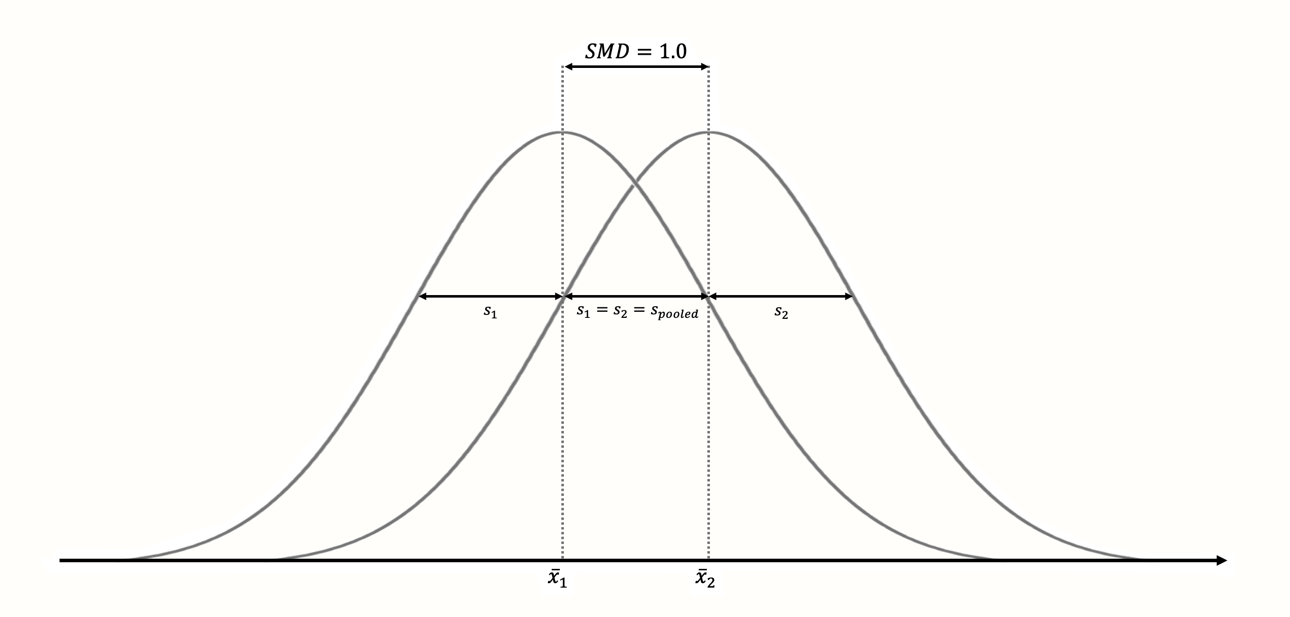
Figure 3.3: Standardized mean difference of 1 (assuming normality, equal standard deviations and equal sample size in both groups).
The standardization makes it much easier to evaluate the magnitude of the mean difference. Standardized mean differences are often interpreted using the conventions by Cohen (1988):
- SMD ≈≈ 0.20: small effect.
- SMD ≈≈ 0.50: moderate effect.
- SMD ≈≈ 0.80: large effect.
Like the convention for Pearson product-moment correlations (Chapter 3.2.3.1), these are rules of thumb at best.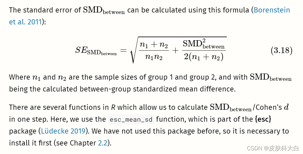
# Load esc package
library(esc)# Define the data we need to calculate SMD/d
# This is just some example data that we made up
grp1m <- 50 # mean of group 1
grp2m <- 60 # mean of group 2
grp1sd <- 10 # sd of group 1
grp2sd <- 10 # sd of group 2
grp1n <- 100 # n of group1
grp2n <- 100 # n of group2# Calculate effect size
esc_mean_sd(grp1m = grp1m, grp2m = grp2m,
grp1sd = grp1sd, grp2sd = grp2sd,
grp1n = grp1n, grp2n = grp2n)
在输出中,有两件事需要提及。首先,我们看到计算出的标准化均值差恰好为 1。这是有道理的,因为我们定义的两个均值之间的差等于(合并的)标准差。
其次,我们看到效应大小是负的。这是因为第 2 组的平均值大于第 1 组的平均值。虽然这在数学上是正确的,但我们有时必须更改计算出的效应大小的符号,以便其他人可以更轻松地解释它们。
想象一下,本例中的数据来自一项研究,测量人们在接受干预(第 1 组)或未接受干预(第 2 组)后每周吸烟的平均数量。在这种情况下,研究结果是积极的,因为干预组的平均吸烟数量较低。因此,将效果大小报告为 1.0 而不是 -1.0 是有意义的,以便其他人可以直观地理解干预具有积极效果。
当一些研究使用的测量值较高意味着更好的结果,而其他研究使用的测量值较低表示更好的结果时,效应大小的符号变得尤为重要。在这种情况下,所有效应大小必须一致地以同一方向编码(例如,我们必须确保在荟萃分析中的所有研究中,较高的效应大小意味着干预组的结果更好)。
通常,小样本校正应用于标准化均值差异,这会产生称为Hedges 的效应大小 G�。我们将在第 3.4.1章中介绍这一更正。
为了对标准化均值差异进行荟萃分析,我们的数据集至少应包含以下列:
n.e。干预/实验组中的观察数量。mean.e。干预/实验组的平均值。sd.e。干预/实验组的标准差。n.c。对照组中的观察数量。mean.c。对照组的平均值。sd.c。对照组的标准差。
3.3.1.3 Within-Group (Standardized) Mean Difference
Within-group unstandardized or standardized mean differences can be calculated when a difference within one group is examined. This is usually the case when the same group of people is measured at two different time points (e.g. before an intervention and after an intervention).

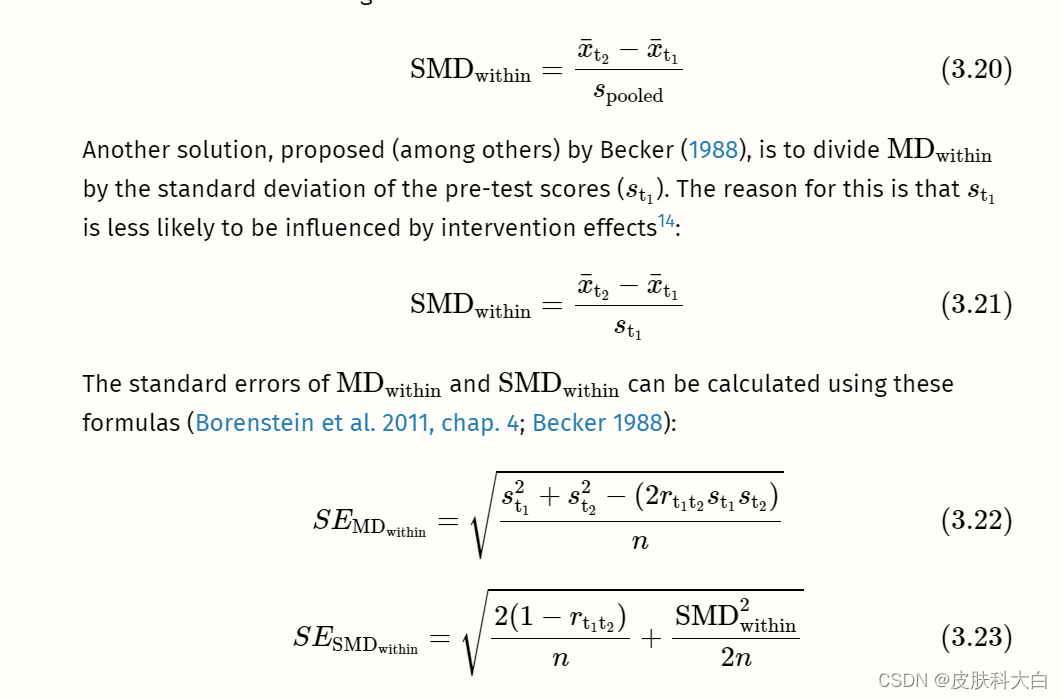

# Define example data needed for effect size calculation
x1 <- 20 # mean at t1
x2 <- 30 # mean at t2
sd1 <- 13 # sd at t1
n <- 80 # sample size
r <- 0.5 # correlation between t1 and t2# Caclulate the raw mean difference
md_within <- x2 - x1# Calculate the smd:
# Here, we use the standard deviation at t1
# to standardize the mean difference
smd_within <- md_within/sd1
smd_within
# Calculate standard error
se_within <- sqrt(((2*(1-r))/n) +
(smd_within^2/(2*n)))
se_within
Meta-analyses of within-group (standardized) mean differences can only be performed in R using pre-calculated effect sizes (see Chapter 3.5.1). The following columns are required in our data set:
TE: The calculated within-group effect size.seTE: The standard error of the within-group effect size.
The Limits of Standardization
Standardized mean differences are, without a doubt, one of the most frequently used effect sizes metrics in meta-analyses. As we mentioned in Chapter 3.3.1.2, standardization allows us, at least in theory, to compare the strength of an effect observed in different studies; even if these studies did not use the same instruments to measure it.
Standardization, however, is not a “Get Out of Jail Free card”. The size of a particular study’s SMDSMD depends heavily on the variability of its sample (see also Viechtbauer 2007a). Imagine that we conduct two identical studies, use the same instrument to measure our outcome of interest, but that the two studies are conducted in two populations with drastically different variances. In this case, the SMDSMD value of both studies would differ greatly, even if the “raw” mean difference in both studies was identical.
In this case, it is somewhat difficult to argue that the “causal” strength of the effect in one study was much larger or smaller than in the other. As Jacob Cohen (1994) put it in a famous paper: “[t]he effect of A on B for me can hardly depend on whether I’m in a group that varies greatly […] or another that does not vary at all” (p. 1001). This problem, by the way, applies to all commonly used “standardized” effect size metrics in meta-analysis, for example correlations.
In addition, we have also seen that the unit by which to standardize is often less clearly defined than one may think. Various options exist both for between- and within-group SMDSMDs, and it is often hard to disentangle which approach was chosen in a particular study. It is necessary to always be as consistent as possible across studies in terms of how we calculate standardized effect sizes for our meta-analysis. Even so, one should keep in mind that the commensurability of effect sizes can be limited, even if standardization was applied.
Of course, the best solution would be if outcomes were measured on the same scale in all studies, so that raw mean differences could be used. In many research fields, however, we are living far away from such a level of methodological harmony. Thus, unfortunately, standardized effect sizes are often our second best option.
.3.2风险与优势比
3.3.2.1风险比率
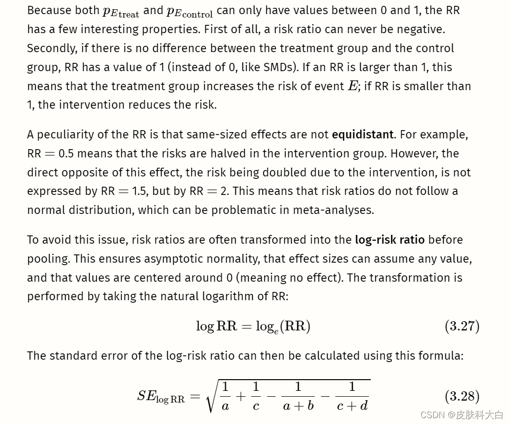
正如其名称所示,风险比(也称为相对风险)是两种风险的比率。风险本质上是比例(参见第3.2.2章)。当我们处理二元或二分结果数据时,可以计算它们。
我们使用“风险”一词而不是“比例”,因为这种类型的结果数据经常出现在医学研究中,在医学研究中检查罹患疾病或死亡的风险。此类事件称为事件。想象一下,我们正在进行一项包含治疗组和对照组的对照临床试验。

# Define data
a <- 46 # events in the treatment group
c <- 77 # events in the control group
n_treat <- 248 # sample size treatment group
n_contr <- 251 # sample size control group# Calculate the risks
p_treat <- a/n_treat
p_contr <- c/n_contr# Calculate the risk ratio
rr <- p_treat/p_contr
rr
# Calculate the log-risk ratio and its standard error
log_rr <- log(rr)
log_rr
se_log_rr <- sqrt((1/a) + (1/c) - (1/n_treat) - (1/n_contr))
se_log_rr
The calculation of risk ratios becomes difficult when there are zero cells. It is possible in practice that a or c (or both) are zero, meaning that no event was recorded in the treatment or control group. If you have a look at the formula used to calculate RRs, it is easy to see why this is problematic. If a (events in the treatment group) is zero, pEtreattreat is also zero, and the RR will be zero. The case of c being zero is even more problematic: it means that pEcontrol control is zero, and we all know that we cannot divide by zero.
通常使用连续性校正来处理这个问题。最常见的连续性校正方法是在所有为零的单元中添加 0.5 的增量(Gart 和 Zweifel 1967)。当对照组和治疗组的样本量很不均匀时,我们还可以使用治疗臂连续性校正 (Sweeting, Sutton, and Lambert 2004).
然而,有证据表明这种修正可能会导致有偏差的结果(Efthimiou 2018)。 (固定效应)Mantel-Haenszel方法是我们将在第 4.2.3.1.1章中发现的一种荟萃分析汇集技术,可以在不进行校正的情况下处理零单元,除非它们存在于我们荟萃分析中的每项研究中。因此,除非适用后一种情况,否则建议避免连续性校正。
零单元问题的一种特殊形式是双零研究。这些研究都涉及A�和C�为零。直觉上,人们可能会认为此类研究的结果仅仅意味着干预组和对照组的风险相似,并且 RR = 1。
不幸的是,事情并不那么容易。两组之间很可能存在真正的效果,但样本量太小而无法检测到这种差异。当概率为乙乙发生率非常低。
想象一下,一位疯狂的科学家进行了一项随机对照试验,其中他评估了氟古里酮(Fulguridone)的效果,这种药物据称可以降低被闪电击中的风险。他将 100 人平均分配到药物组或对照组,并观察他们三年。试验结果令人失望,因为无论是治疗组还是对照组,都没有人被闪电击中。然而,我们知道,一般来说,被闪电击中的可能性有多大。仅观察 100 个人根本不足以发现这种罕见事件中的差异,即使我们接受治疗有效这一有点奇怪的想法。因此,在汇总效应时,双零研究通常被完全丢弃。
这导致我们对风险比率提出最后一个警告:它们没有向我们提供有关事件总体上有多常见的信息。例如,如果荟萃分析报告的风险比为 0.5,我们就知道干预措施可以将风险降低一半。但我们不知道它是否将风险从 40% 降低到 20%,或者从 0.004% 降低到 0.002%。风险比率是否具有实际意义取决于具体情况。如果风险比 0.5 代表风险降低 0.002%,这可能不会对人口水平产生很大影响,但如果感兴趣的事件是例如严重且使人衰弱的疾病,则它可能仍然很重要。
当我们在R中进行荟萃分析时,通常不需要手动计算研究的对数风险比。导入数据时我们也不必担心零单元格。我们的数据集中应包含以下列:
event.e。治疗组或实验组中的事件数。n.e。治疗组或实验组的样本量。event.c。对照组中的事件数。n.c。对照组的样本量。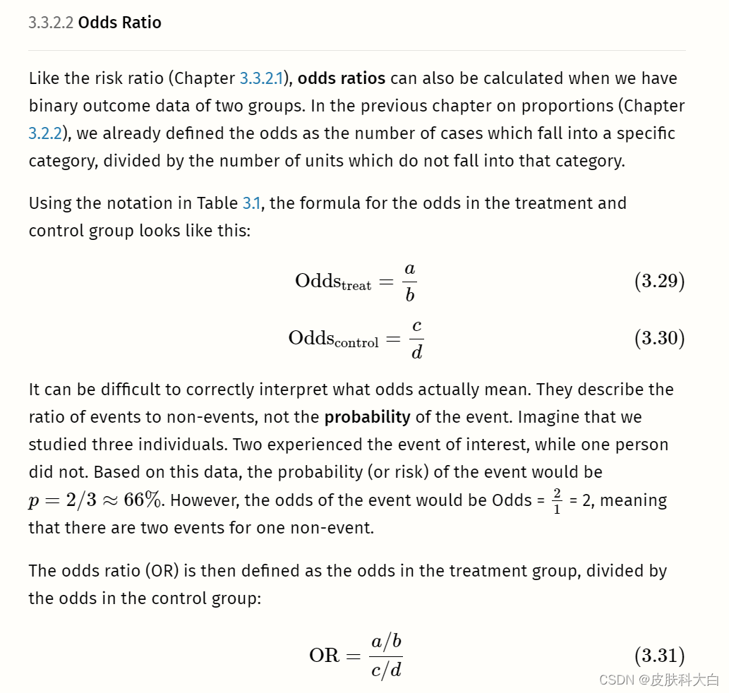
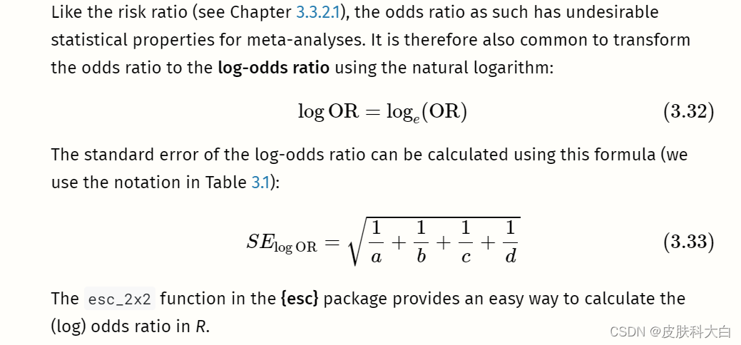
library(esc)
# Define data
grp1yes <- 45 # events in the treatment group
grp1no <- 98 # non-events in the treatment group
grp2yes <- 67 # events in the control group
grp2no <- 76 # non-events in the control group# Calculate OR by setting es.type to "or"
esc_2x2(grp1yes = grp1yes, grp1no = grp1no,
grp2yes = grp2yes, grp2no = grp2no,
es.type = "or")
# Calculate logOR by setting es.type to "logit"
esc_2x2(grp1yes = grp1yes, grp1no = grp1no,
grp2yes = grp2yes, grp2no = grp2no,
es.type = "logit")
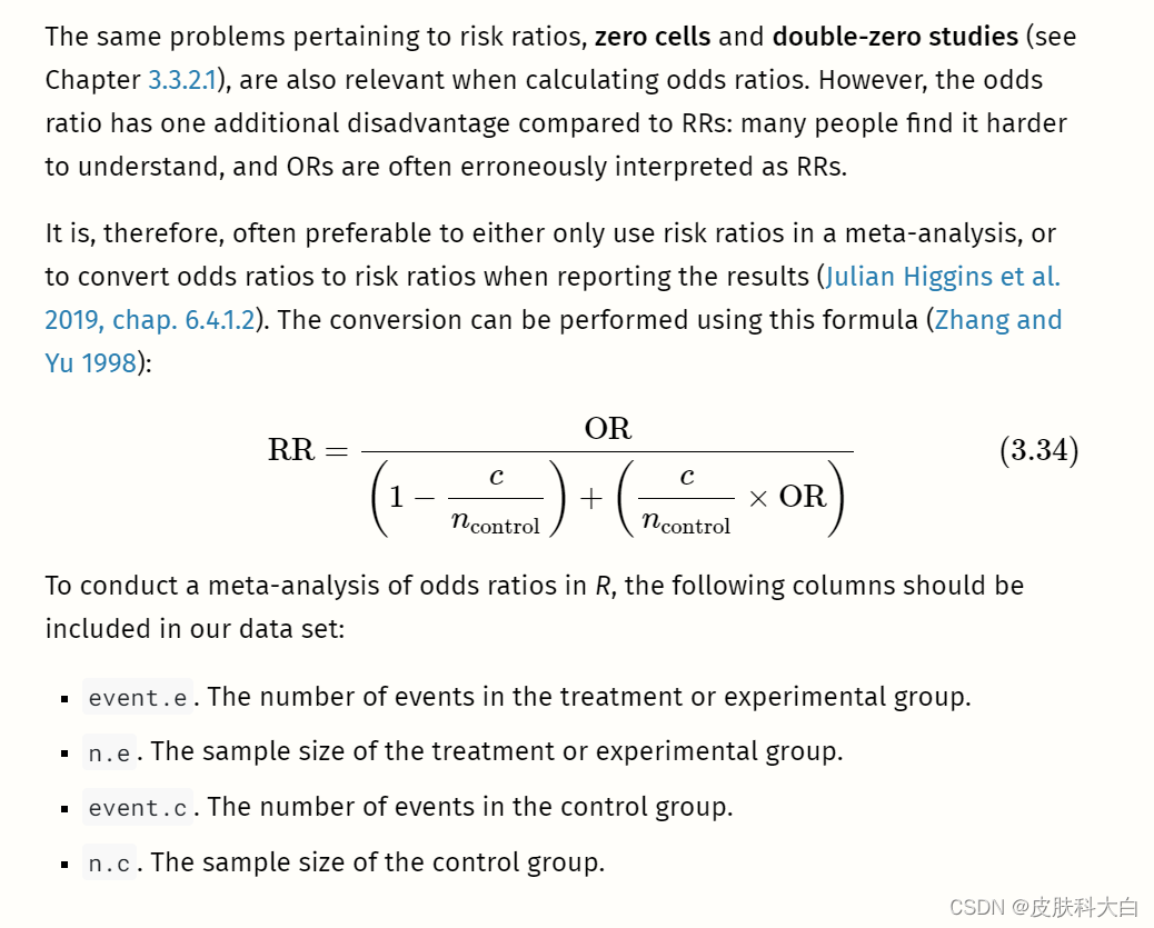
3.3.3 Incidence Rate Ratios
The effect sizes for binary outcome data we examined previously, risk ratios and odds ratios, are ways to compare the number of events in two groups. However, they do not directly encode the time during which these events occurred. When calculating a risk or odds ratio, we tacitly assume that the observation periods in both groups are comparable. Furthermore, risk and odds ratios do not provide us with any information on how long it took until the events occurred.
In some cases, this is just fine, because the time frame is not overly relevant for our research question. It is also possible that our binary data is cross-sectional and has no time dimension at all15. In these cases, the risk or odds ratio is usually an appropriate effect size metric.
But now, imagine a study in which we examine the mortality of individuals in two groups over 10 years. It might be possible that the number of events over these 10 years (e.g. death) is roughly similar in both groups. However, once we have a closer look at when the deaths occurred, we see that more events in one group occurred in the first years, while in the other group, somewhat more events occurred to the end of our 10-year observation period. The calculated odds or risk ratio for our data would be approximately 1, indicating no group difference. But this misses something important: that participants in one group survived somewhat longer, even if they died eventually.
To incorporate time into our effect size estimate, we can calculate incidence rate ratios, which are sometimes simply called rate ratios. Incidence rate ratios consist of two incidence rates. To calculate these incidence rates, we have to first understand the concept of person-time.
The person-time expresses the total time in which participants in a study were at risk of having an event. To calculate the person-time, we sum up the time at risk (expressed as days, weeks, or years) of all study subjects. However, the time at risk differs from person to person.
To exemplify this, imagine we are conducting a study with 6 participants. The study lasts for exactly 10 years. After each year, we interview the participants to examine if they experienced the event of interest. Whenever we observe that the event has occurred, the study ends for the affected participant, and we do not examine her or him until the study ends. The results of our study are visualized in Figure 3.4.
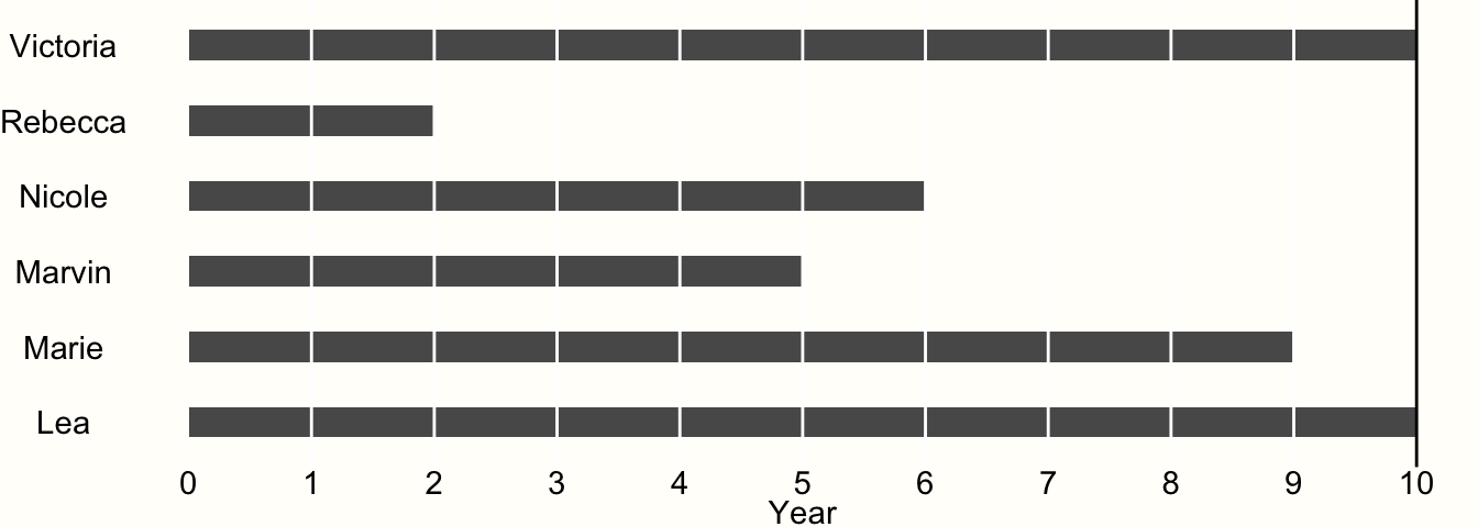
Figure 3.4: Example of time-to-event data.
We see that only two of our participants, Victoria and Lea, remained in the study until the end. This is because they did not experience the event during the entire 10-year observation period. Therefore, both were at risk for 10 years.
All other participants experienced the event during the study period. When Rebecca was examined at year 2, for example, we found out that she experienced the event during the last year. However, we only know that the event occurred during year 2, not when exactly.
Research data like this is called interval censored data, and very frequently found in clinical trials which conduct a so-called survival analysis. Data being censored means that we only partially know how long Rebecca was at risk before she finally experienced the event. We know that she had the event after year 1 and before the end of year 2, but not more. Lacking other information, we may therefore assume that the event occurred somewhere in the middle, and settle with a time at risk of 1.5 years.
If we apply the same scheme for all our censored data, we can calculate the person-years at risk in our study:
10+1.5+5.5+4.5+8.5+10=4010+1.5+5.5+4.5+8.5+10=40So the estimated total person-years at risk in our study is 40. Knowing that a year has 52 weeks, we can also calculate the person-weeks of our study: 40×52=208040×52=2080.
Now that we know the person-years in our experiment, which we will denote as T�, we can also calculate the incidence rate within one year. We know that four participants experienced the event during the study period, so the number of events is E=4�=4. We can then calculate the incidence rate IR using this formula: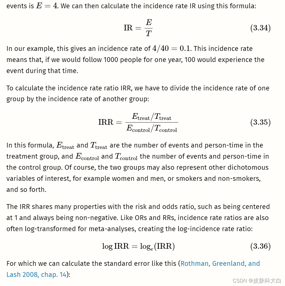

In this example, we simulated a case in which the number of events Etreat�treat and Econtrol�control is exactly equal, but where the treatment group has a longer person-time at risk. This time difference is accounted for when we calculate IRRs. Therefore, the result we get is not 1, but IRR ≈≈ 0.79, indicating that the incidence rate is smaller in the treatment group.
Incidence rate ratios are commonly used in epidemiology and prevention research. They can be used when participants are followed for a longer period of time, and when there are regular assessments in between. In practice, however, there is one caveat we should consider when calculating IRRs as part of a meta-analysis: it is important that the incidence data reported in the included articles is fine-grained enough. Sometimes, papers only report the total number of events during the entire study period and not the number of events recorded at each assessment point in between. It is also possible that no interim assessments were made to begin with.
In our example above (see Figure 3.4), we simply took the midpoint between the last “event-free” assessment point and the assessment point in which the event was recorded to estimate the time at risk of a participant. It is important to keep in mind that this is only a best guess of when the event happened exactly. Even when taking the midpoint, our estimates can still be off by about half a year in our example.
Our estimate of the person-time will be best if the time between assessment points is as small as possible. If assessment intervals in a study are too coarse depends on the context of the meta-analysis, but it is always advisable to conduct sensitivity analyses (Panageas et al. 2007).
This means to recalculate the IRR of studies based on different estimates of the person-time:
-
using the midpoint of the interval,
-
using the last “event-free” assessment point, and
-
using the assessment point in which the event was detected.
If the results of all three of these meta-analyses point in the same direction, we can be more confident in our findings. We should also make sure that the assessment periods do not differ too much between studies (e.g. one study examining events daily, and the other only each year). When there are doubts about the applicability of IRRs for a meta-analysis, there is always the possibility to calculate risk or odds ratios instead (or in addition). However, when we do this, we should make sure that the assessment point was similar in each study (e.g. after one year).
To calculate a meta-analysis based on incidence rate ratios in R, the following columns need to be prepared in our data set:
event.e: The total number of events in the treatment or experimental group.time.e: The person-time in the treatment or experimental group. The person-time has to be expressed in the same units (person-days, person-weeks, or person-years) in all studies.event.c: The total number of events in the control group.time.c: The person-time in the control group. The person-time has to be expressed in the same units (person-days, person-weeks, or person-years) in all studies.
相关文章:

荟萃分析R Meta-Analyses 3 Effect Sizes
总结 效应量是荟萃分析的基石。为了进行荟萃分析,我们至少需要估计效应大小及其标准误差。 效应大小的标准误差代表研究对效应估计的精确程度。荟萃分析以更高的精度和更高的权重给出效应量,因为它们可以更好地估计真实效应。 我们可以在荟萃分析中使用…...

常用的8个应用和中间件的Docker运行示例
文章目录 1、Docker Web 管理工具 portainer2、在线代码编辑器 Code Server3、MySQL4、Redis5、Nginx6、PostgreSQL7、媒体管理工具 Dim8、Gitlab 1、Docker Web 管理工具 portainer Portainer 是一个轻量级的管理 UI ,可让你轻松管理不同的 Docker 环境࿰…...

UnoCSS实现背景图片样式加载
UnoCSS是一个好东西,可以把任何style样式通过css去描述。但是默认使用的tailwindcss有一个不完美,就是当使用图片时,背景图片无法通过原子化css直接描述。例如有一个背景图片,则必须为该图片单独出一个css样式,然后再加…...
vue前端工程化
前言 本文介绍的是有关于vue方面的前端工程化实践,主要通过实践操作让开发人员更好的理解整个前端工程化的流程。 本文通过开发准备阶段、开发阶段和开发完成三个阶段开介绍vue前端工程化的整体过程。 准备阶段 准备阶段我将其分为:框架选择、规范制…...

面向对象:继承
文章目录 一、什么叫继承?二、单继承三、多继承3.1多继承的各种情况3.1.1一般情况3.1.1特殊情况(菱形继承) 四、菱形继承引发的问题4.1 问题1:数据冗余4.2 问题2:二义性(无法确定到底是访问哪个) 五、虚拟继承解决菱形…...
ES学习日记(一)-------单节点安装启动
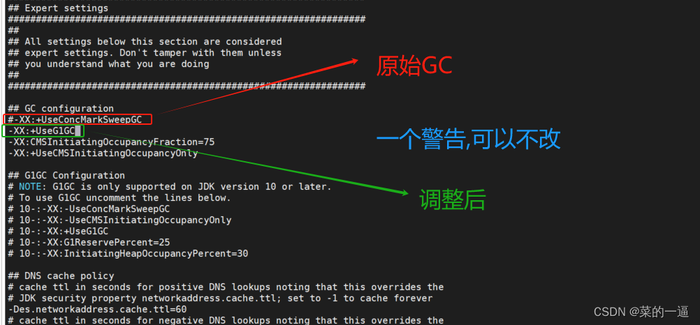
基于ES7.4.1编写,其实一开始用的最新的8.1,但是问题太多了!!!!不稳定,降到7.4 下载好的安装包上传到服务器或虚拟机,创建ES目录,命令mkdir -p /路径xxxx 复制安装包到指定路径并解压: tar zxvf elasticsearch-8.1.0-linux-x86_64.tar.gz -C /usr/local/es/ 进入bin目录安装,命…...

【管理咨询宝藏59】某大型汽车物流战略咨询报告
本报告首发于公号“管理咨询宝藏”,如需阅读完整版报告内容,请查阅公号“管理咨询宝藏”。 【管理咨询宝藏59】某大型汽车物流战略咨询报告 【格式】PDF 【关键词】HR调研、商业分析、管理咨询 【核心观点】 - 重新评估和调整商业模式,开拓…...
ArcGIS Pro横向水平图例
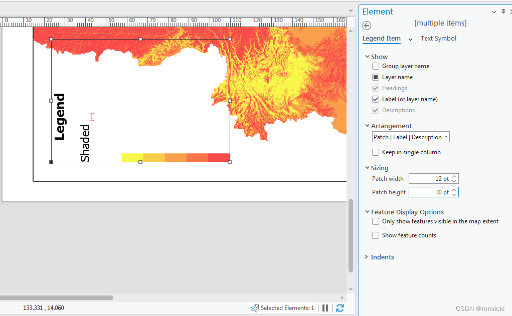
终于知道ArcGIS Pro怎么调横向图例了! 简单的像0一样 旋转,左转右转随便转 然后调整图例项间距就可以了,参数太多就随便试,总有一款适合你! 要调整长度,就调整图例块的大小。完美! 好不容易…...

线程创建的几种方式
1.继承Thread类 class MyThread extends Thread {public void run() {// 线程执行的任务for (int i 0; i < 5; i) {System.out.println("Thread: " i);try {Thread.sleep(1000); // 使线程休眠 1 秒} catch (InterruptedException e) {e.printStackTrace();}}}…...
)
Python教程:一文掌握Python多线程(很详细)
目录 1.什么是多线程? 1.1多线程与单线程的区别 1.2 Python 中的多线程实现方式 2.使用 threading 模块创建和管理线程 2.1创建线程:Thread 类的基本用法 2.2线程的启动和执行:start() 方法 2.3线程的同步和阻塞:join() 方…...

华为防火墙配置指引超详细(包含安全配置部分)以USG6320为例
华为防火墙USG6320 华为防火墙USG6320是一款高性能、高可靠的下一代防火墙,适用于中小型企业、分支机构等场景。该防火墙支持多种安全功能,可以有效抵御网络攻击,保护网络安全。 目录 华为防火墙USG6320 1. 初始配置 2. 安全策略配置 3. 防火墙功能配置 4. 高可用性配…...
固定在左上方某盒子内(如按钮)添加可拖动功能,使用react hook语法实现)
(含react-draggable库以及相关BUG如何解决)固定在左上方某盒子内(如按钮)添加可拖动功能,使用react hook语法实现
原生写法 // 封装组件 import React, { useState, useRef } from react;const DraggableModal ({ children }) > {const [position, setPosition] useState({ x: 0, y: 0 });const modalRef useRef(null);const handleMouseDown (e) > {const modal modalRef.curre…...

选择最佳图像处理工具OpenCV、JAI、ImageJ、Thumbnailator和Graphics2D
文章目录 1、前言2、 图像处理工具效果对比2.1 Graphics2D实现2.2 Thumbnailator实现2.3 ImageJ实现2.4 JAI(Java Advanced Imaging)实现2.5 OpenCV实现 3、图像处理工具结果 1、前言 SVD(stable video diffusion)开放了图生视频的API,但是限…...

微信小程序版本更新检测
app.vue文件 <script>export default {onLaunch: function() {console.log(App Launch)// #ifdef MP-WEIXINthis.getUpdateManager();// #endif},methods: {// 检测小程序更新getUpdateManager() {const updateManager wx.getUpdateManager();updateManager.onCheckFor…...

【每日力扣】343. 整数拆分与63. 不同路径 II
🔥 个人主页: 黑洞晓威 😀你不必等到非常厉害,才敢开始,你需要开始,才会变的非常厉害 343. 整数拆分 给定一个正整数 n ,将其拆分为 k 个 正整数 的和( k > 2 ),并使…...

洛谷 Cut Ribbon
思路:我们可以看出,这是一道完全背包问题,但是呢,有一点需要注意:那就是我们在装背包的时候并不能保证一定能装满背包,但是这里的背包要求是让我们装满的,所以我们需要判断这个背包装满才行&…...

#AS,idea,maven,gradle
Jdk,sdk。提前都是需要下好的。 Maven与gradle的思考: 用AS开发app时,gradle本就有,自己也可以指定,AGP同样。要注意gradle,AGP,jdk版本的事情。还有依赖库。 用idea开发网络程序时,也有内置的maven&…...
FPGA结构与片上资源
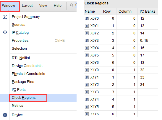
文章目录 0.总览1.可配置逻辑块CLB1.1 6输入查找表(LUT6)1.2 选择器(MUX)1.3 进位链(Carry Chain)1.4 触发器(Flip-Flop) 2.可编程I/O单元2.1 I/O物理级2.2 I/O逻辑级 3.布线资源4.其…...

【分布式】——分布式事务
分布式事务 ⭐⭐⭐⭐⭐⭐ Github主页👉https://github.com/A-BigTree 笔记链接👉https://github.com/A-BigTree/tree-learning-notes ⭐⭐⭐⭐⭐⭐ Spring专栏👉https://blog.csdn.net/weixin_53580595/category_12279588.html SpringMVC专…...

第6章:“让我们思考这个”的提示
“让我们思考这个”这一提示词,是深度对话的钥匙,鼓励ChatGPT生成反思性、沉思性的文本。 对于论文写作、诗歌创作或创意任务的完成,非常实用。 当你想要深究某主题时,只需向ChatGPT提问。 它会基于提示,结合算法和…...
)
网络爬虫主流思路及反爬破解技术应用(新手速成)
网络爬虫的主流思路是模拟浏览器行为自动化抓取网页数据,而反爬破解技术则通过代理IP、请求伪装、动态渲染处理等方式绕过网站防护机制,实现稳定高效的数据采集 。一、主流爬虫技术思路 1.请求模拟与数据提取 使用 requests 或 urllib 构建H…...

DAMO-YOLO在Vue前端项目中的实时检测应用
DAMO-YOLO在Vue前端项目中的实时检测应用 1. 引言 想象一下,你正在开发一个智能安防系统,需要在网页上实时检测监控视频中的人员和车辆。传统的方案是将视频流发送到服务器处理,但网络延迟和隐私问题让人头疼。有没有可能在用户的浏览器里直…...
)
深入浅出:从原理到实践,手把手教你理解并校准RV1126 ISP的黑电平(BLC)
深入浅出:从原理到实践,手把手教你理解并校准RV1126 ISP的黑电平(BLC) 在数字图像处理领域,黑电平校准(Black Level Calibration, BLC)是一个看似简单却至关重要的环节。想象一下,当你用专业相机拍摄星空时…...

Fish-Speech 1.5效果展示:双自回归Transformer架构,语音质量惊艳
Fish-Speech 1.5效果展示:双自回归Transformer架构,语音质量惊艳 你听过那种一听就知道是机器人的AI语音吗?生硬、刻板,每个字都像从模板里抠出来的,毫无生气。再听听这个:“今天天气真好,适合…...
)
避开理论深坑:给开发者的机器学习实用入门指南(附周志华《机器学习》高效阅读路线)
避开理论深坑:给开发者的机器学习实用入门指南 作为一名开发者,你可能已经意识到机器学习正在改变我们解决问题的方式。从推荐系统到图像识别,从自然语言处理到预测分析,机器学习正在成为现代软件开发不可或缺的一部分。但当你翻开…...

SolveSpace:参数化 CAD 软件网页版的实验性突破
【导语:SolveSpace 作为一款参数化二维/三维 CAD 软件,推出了实验性网页版。虽存在速度损失和未解决的 bug,但处理小模型时体验不错,为 CAD 软件的使用带来新可能。】小巧 CAD 软件的网页版尝试SolveSpace 主要以普通桌面软件形式…...

Qwen3.5-4B-Claude-Opus保姆级教程:Web端UI功能分区与高级参数联动说明
Qwen3.5-4B-Claude-Opus保姆级教程:Web端UI功能分区与高级参数联动说明 1. 模型与平台介绍 Qwen3.5-4B-Claude-4.6-Opus-Reasoning-Distilled-GGUF 是一个基于 Qwen3.5-4B 的推理蒸馏模型,重点强化了结构化分析、分步骤回答、代码与逻辑类问题的处理能…...

终极解决方案:5分钟完成DOCX到LaTeX的专业转换指南 [特殊字符]
终极解决方案:5分钟完成DOCX到LaTeX的专业转换指南 🚀 【免费下载链接】docx2tex Converts Microsoft Word docx to LaTeX 项目地址: https://gitcode.com/gh_mirrors/do/docx2tex 还在为Word文档转换LaTeX格式而烦恼吗?docx2tex就是你…...

二手交易平台信任度调查:闲鱼交易安全性深度解析
二手交易平台信任度调查:闲鱼交易安全性深度解析随着循环经济的兴起,中国二手交易市场规模在2023年突破万亿元大关。作为阿里巴巴旗下的C2C二手交易平台,闲鱼凭借5亿注册用户和日均10亿元的交易规模,已成为国内最大的闲置物品流转…...

别再手动画封装了!用嘉立创EDA免费库5分钟搞定Altium Designer缺失的器件
5分钟极速救援:用嘉立创EDA破解Altium Designer封装缺失难题 深夜11点,李工盯着屏幕上闪烁的光标和半成品的PCB布局图,额头渗出细密的汗珠。项目交付截止前48小时,团队突然发现Altium Designer官方库中缺少关键芯片TPS5430DDAR的封…...
