python tensorflow 各种神经元
-
感知机神经元(Perceptron Neuron):
-
最基本的人工神经元模型,用于线性分类任务。
import numpy as npclass Perceptron:def __init__(self, input_size, learning_rate=0.01, epochs=1000):self.weights = np.zeros(input_size + 1)  # 加上一个偏置self.learning_rate = learning_rateself.epochs = epochsdef activation(self, x):return 1 if x >= 0 else 0def predict(self, x):summation = np.dot(x, self.weights[1:]) + self.weights[0]return self.activation(summation)def train(self, training_inputs, labels):for _ in range(self.epochs):for inputs, label in zip(training_inputs, labels):prediction = self.predict(inputs)self.weights[1:] += self.learning_rate * (label - prediction) * inputsself.weights[0] += self.learning_rate * (label - prediction)# 示例数据
training_inputs = np.array([[1, 1], [1, 0], [0, 1], [0, 0]])
labels = np.array([1, 0, 0, 0])# 创建感知机实例并训练
perceptron = Perceptron(input_size=2)
perceptron.train(training_inputs, labels)# 测试感知机
inputs = np.array([1, 1])
print("Input:", inputs, "Prediction:", perceptron.predict(inputs))inputs = np.array([0, 0])
print("Input:", inputs, "Prediction:", perceptron.predict(inputs))
代码解释
- 类定义:
Perceptron类包含了初始化函数、激活函数、预测函数和训练函数。 - 初始化: 初始化权重为零,并设置学习率和训练轮数。
- 激活函数: 使用阶跃函数(step function)作为激活函数。
- 预测函数: 计算输入和权重的加权和,然后通过激活函数得到输出。
- 训练函数: 使用感知机学习规则,迭代更新权重。
- 示例数据: 二分类数据集(逻辑与问题)。
- 训练与测试: 训练感知机并测试其对新输入的预测。
- 类定义:
-
-
多层感知机神经元(Multi-Layer Perceptron, MLP):
-
包含多个隐藏层的感知机,能够学习复杂的非线性关系。
-
使用一个简单的MLP模型来处理二分类任务。
import numpy as npfrom keras.models import Sequential
from keras.layers import Dense# 生成示例数据
# 输入数据:4个样本,每个样本2个特征
training_inputs = np.array([[0, 0], [0, 1], [1, 0], [1, 1]])
# 标签:与XOR逻辑相符的二分类标签
labels = np.array([[0], [1], [1], [0]])# 创建MLP模型
model = Sequential()
model.add(Dense(4, input_dim=2, activation='relu'))  # 隐藏层,包含4个神经元,ReLU激活函数
model.add(Dense(1, activation='sigmoid'))  # 输出层,1个神经元,sigmoid激活函数用于二分类# 编译模型
model.compile(loss='binary_crossentropy', optimizer='adam', metrics=['accuracy'])# 训练模型
model.fit(training_inputs, labels, epochs=1000, verbose=0)# 测试模型
test_inputs = np.array([[0, 0], [0, 1], [1, 0], [1, 1]])
predictions = model.predict(test_inputs)# 输出测试结果
for i, test_input in enumerate(test_inputs):print(f"Input: {test_input}, Predicted: {predictions[i][0]:.4f}")
代码解释
- 库导入: 导入必要的库,包括
numpy用于数据处理,Sequential用于构建模型,Dense用于构建层。 - 数据准备: 创建一个简单的XOR逻辑问题的数据集。
- 模型构建:
- 使用
Sequential构建模型。 - 添加一个隐藏层,包含4个神经元,使用ReLU激活函数。
- 添加一个输出层,包含1个神经元,使用sigmoid激活函数(适合二分类任务)。
- 使用
- 模型编译: 使用二元交叉熵损失函数和Adam优化器进行编译,并指定准确率为评估指标。
- 模型训练: 训练模型1000个轮次,设置
verbose=0以抑制训练期间的详细输出。 - 模型测试: 使用训练好的模型对测试数据进行预测,并输出结果。
- 库导入: 导入必要的库,包括
-
-
卷积神经网络神经元(Convolutional Neural Network, CNN):
-
专门用于处理图像数据,通过卷积层提取空间特征。
-
构建一个简单的 RNN 来处理时间序列数据,例如序列预测任务。
from keras.models import Sequential
from keras.layers import SimpleRNN, Dense
import numpy as np# 生成示例数据
# 假设有一个时间序列数据集,每个序列长度为5,特征数量为1
X = np.array([[[0.0], [1.0], [2.0], [3.0], [4.0]],[[1.0], [2.0], [3.0], [4.0], [5.0]],[[2.0], [3.0], [4.0], [5.0], [6.0]],
])
y = np.array([5.0, 6.0, 7.0])# 创建 RNN 模型
model = Sequential()
model.add(SimpleRNN(10, activation='relu', input_shape=(5, 1)))
model.add(Dense(1))# 编译模型
model.compile(optimizer='adam', loss='mse')# 训练模型
model.fit(X, y, epochs=200, verbose=0)# 预测
new_sequence = np.array([[[3.0], [4.0], [5.0], [6.0], [7.0]]])
prediction = model.predict(new_sequence)
print("Predicted value:", prediction)
代码解释
- 导入必要的库:使用 TensorFlow 和 Keras 来构建和训练 RNN 模型,同时用 NumPy 生成示例数据。
- 生成示例数据:创建一个时间序列数据集
X和相应的目标值y。 - 创建模型:使用
Sequential模型构建一个包含一个SimpleRNN层和一个Dense层的简单 RNN 模型。 - 编译模型:使用
adam优化器和均方误差损失函数编译模型。 - 训练模型:用示例数据训练模型 200 个 epochs。
- 进行预测:用训练好的模型对一个新的时间序列进行预测。
-
-
循环神经网络神经元(Recurrent Neural Network, RNN):
-
能够处理序列数据,具有记忆功能,适用于时间序列分析、语言模型等。
-
使用RNN处理序列数据。将创建一个模型来预测给定序列的下一个数字。
import tensorflow as tf
from keras.models import Sequential
from keras.layers import SimpleRNN, Dense
import numpy as np# 生成示例数据
# 假设有一个时间序列数据集,每个序列长度为5,特征数量为1
X = np.array([[[0.0], [1.0], [2.0], [3.0], [4.0]],[[1.0], [2.0], [3.0], [4.0], [5.0]],[[2.0], [3.0], [4.0], [5.0], [6.0]],
])
y = np.array([5.0, 6.0, 7.0])# 创建 RNN 模型
model = Sequential()
model.add(SimpleRNN(10, activation='relu', input_shape=(5, 1)))
model.add(Dense(1))# 编译模型
model.compile(optimizer='adam', loss='mse')# 训练模型
model.fit(X, y, epochs=200, verbose=0)# 预测
new_sequence = np.array([[[3.0], [4.0], [5.0], [6.0], [7.0]]])
prediction = model.predict(new_sequence)
print("Predicted value:", prediction)
代码解释
- 数据生成与准备:
generate_sequence(): 生成一个简单的序列。prepare_data(): 准备训练数据,将序列转换为模型可以接受的格式。
- 模型构建:
- 使用
Sequential构建模型。 - 添加一个
SimpleRNN层,包含10个神经元,输入形状由数据决定,return_sequences=True表示输出每个时间步的结果。 - 添加一个
Dense层作为输出层,预测序列的下一个值。
- 使用
- 模型编译: 使用均方误差作为损失函数,使用Adam优化器。
- 模型训练: 训练模型1000个轮次,
verbose=0表示不显示训练过程中的详细信息。 - 模型测试: 使用模型预测给定序列的下一个值。
- 数据生成与准备:
-
-
长短期记忆网络神经元(Long Short-Term Memory, LSTM):
-
RNN的一种,通过门控机制解决长期依赖问题,适合处理长序列数据。
-
长一个简单的LSTM模型示例,用于预测时间序列数据。
import numpy as np
from keras.models import Sequential
from keras.layers import LSTM, Dense
from  sklearn.preprocessing import MinMaxScaler
import matplotlib.pyplot as plt# 生成示例数据
np.random.seed(0)
data = np.sin(np.linspace(0, 100, 1000)) + np.random.normal(scale=0.5, size=1000)# 数据预处理
scaler = MinMaxScaler(feature_range=(0, 1))
scaled_data = scaler.fit_transform(data.reshape(-1, 1))# 创建训练和测试数据集
train_size = int(len(scaled_data) * 0.8)
train, test = scaled_data[:train_size], scaled_data[train_size:]# 创建数据集函数
def create_dataset(data, time_step=1):X, Y = [], []for i in range(len(data) - time_step - 1):a = data[i:(i + time_step), 0]X.append(a)Y.append(data[i + time_step, 0])return np.array(X), np.array(Y)time_step = 10
X_train, y_train = create_dataset(train, time_step)
X_test, y_test = create_dataset(test, time_step)# Reshape input to be [samples, time steps, features] which is required for LSTM
X_train = X_train.reshape(X_train.shape[0], X_train.shape[1], 1)
X_test = X_test.reshape(X_test.shape[0], X_test.shape[1], 1)# 创建LSTM模型
model = Sequential()
model.add(LSTM(50, return_sequences=True, input_shape=(time_step, 1)))
model.add(LSTM(50, return_sequences=False))
model.add(Dense(1))
model.compile(optimizer='adam', loss='mean_squared_error')# 训练模型
model.fit(X_train, y_train, epochs=20, batch_size=32, verbose=1)# 预测
train_predict = model.predict(X_train)
test_predict = model.predict(X_test)# 逆缩放预测值
train_predict = scaler.inverse_transform(train_predict)
test_predict = scaler.inverse_transform(test_predict)
y_train = scaler.inverse_transform(y_train.reshape(-1, 1))
y_test = scaler.inverse_transform(y_test.reshape(-1, 1))# 可视化结果
plt.figure(figsize=(14, 8))
plt.plot(data, label='True Data')
train_predict_plot = np.empty_like(data)
train_predict_plot[:] = np.nan
train_predict_plot[time_step:len(train_predict) + time_step] = train_predict[:, 0]
plt.plot(train_predict_plot, label='Train Predict')test_predict_plot = np.empty_like(data)
test_predict_plot[:] = np.nan
test_predict_plot[len(train_predict) + (time_step * 2) + 1:len(data) - 1] = test_predict[:, 0]
plt.plot(test_predict_plot, label='Test Predict')plt.xlabel('Time')
plt.ylabel('Value')
plt.legend()
plt.show()
-
-
门控循环单元神经元(Gated Recurrent Unit, GRU):
-
类似于LSTM,但结构更简单,参数更少,也用于处理序列数据。
-
使用TensorFlow实现的简单门控循环单元(Gated Recurrent Unit, GRU),定义一个简单的GRU模型,并训练它来处理序列数据。
import tensorflow as tf
from keras.models import Sequential
from keras.layers import GRU, Dense
import numpy as np# 定义超参数
input_size = 10   # 输入特征的维度
hidden_size = 20  # 隐藏层神经元数量
output_size = 1   # 输出的维度
num_epochs = 100  # 训练的迭代次数
learning_rate = 0.01  # 学习率# 生成一些假数据
sequence_length = 5  # 每个序列的长度
batch_size = 3       # 每批次的数据量
x = np.random.randn(batch_size, sequence_length, input_size).astype(np.float32)  # 随机输入数据
y = np.random.randn(batch_size, output_size).astype(np.float32)  # 随机输出数据# 定义GRU模型
model = Sequential()
model.add(GRU(hidden_size, input_shape=(sequence_length, input_size), return_sequences=False))
model.add(Dense(output_size))# 编译模型
model.compile(optimizer=tf.keras.optimizers.Adam(learning_rate=learning_rate), loss='mse')# 训练模型
history = model.fit(x, y, epochs=num_epochs, verbose=1)print('Training complete.')
这个代码示例展示了如何定义一个简单的GRU模型,并使用TensorFlow对其进行训练。以下是关键步骤的解释:
-
定义超参数:设置输入特征的维度、隐藏层神经元数量、输出维度、训练迭代次数和学习率。
-
生成假数据:使用随机数生成器创建一些输入和输出数据来模拟训练数据,并转换为浮点数类型。
-
定义GRU模型:使用
Sequential模型,添加一个GRU层和一个全连接层。GRU层使用GRU,全连接层使用Dense。 -
编译模型:使用Adam优化器,并设置均方误差(MSE)为损失函数。
-
训练模型:使用
fit方法进行训练,传入输入数据和目标数据,设置训练的迭代次数,并打印训练过程。
-
-
-
径向基函数神经元(Radial Basis Function, RBF Neuron):
-
使用径向基函数作为激活函数,常用于模式识别和函数逼近。
-
import tensorflow as tf
import numpy as np# Define the Radial Basis Function (RBF) layer
class RBFLayer(tf.keras.layers.Layer):def __init__(self, units, gamma):super(RBFLayer, self).__init__()self.units = unitsself.gamma = tf.constant(gamma, dtype=tf.float32)def build(self, input_shape):self.mu = self.add_weight(shape=(self.units, input_shape[-1]),initializer='random_normal',trainable=True,name='mu')def call(self, inputs):diff = tf.expand_dims(inputs, axis=1) - tf.expand_dims(self.mu, axis=0)sq_diff = tf.reduce_sum(tf.square(diff), axis=-1)return tf.exp(-self.gamma * sq_diff)# Example of using RBFLayer in a model
def create_model(input_dim, rbf_units, gamma):model = tf.keras.Sequential([tf.keras.layers.InputLayer(input_shape=(input_dim,)),RBFLayer(units=rbf_units, gamma=gamma),tf.keras.layers.Dense(1)  # Example output layer, you can adjust this as needed])return model# Create some example data
np.random.seed(0)
X_train = np.random.randn(100, 2)
y_train = np.random.randn(100, 1)# Parameters
input_dim = 2
rbf_units = 10
gamma = 1.0# Create and compile the model
model = create_model(input_dim, rbf_units, gamma)
model.compile(optimizer='adam', loss='mse')# Train the model
model.fit(X_train, y_train, epochs=100, verbose=0)# Predict
predictions = model.predict(X_train)
print(predictions)
-
-
自编码器神经元(Autoencoder Neuron):
-
用于数据压缩和特征学习,通过编码和解码过程学习数据的有效表示。
-
使用TensorFlow库实现自编码器神经元,使用MNIST数据集。
import tensorflow as tf
from keras import layers, losses
from keras.models import Model
from keras.datasets import mnist
import numpy as np# 加载MNIST数据集
(x_train, _), (x_test, _) = mnist.load_data()# 归一化数据
x_train = x_train.astype('float32') / 255.
x_test = x_test.astype('float32') / 255.# 扁平化数据
x_train = x_train.reshape((len(x_train), np.prod(x_train.shape[1:])))
x_test = x_test.reshape((len(x_test), np.prod(x_test.shape[1:])))# 定义编码器
class Autoencoder(Model):def __init__(self, encoding_dim):super(Autoencoder, self).__init__()self.encoding_dim = encoding_dimself.encoder = tf.keras.Sequential([layers.Dense(encoding_dim, activation='relu'),])self.decoder = tf.keras.Sequential([layers.Dense(784, activation='sigmoid')])def call(self, x):encoded = self.encoder(x)decoded = self.decoder(encoded)return decoded# 初始化自编码器模型
autoencoder = Autoencoder(32)# 编译模型
autoencoder.compile(optimizer='adam', loss=losses.MeanSquaredError())# 训练模型
autoencoder.fit(x_train, x_train,epochs=10,shuffle=True,validation_data=(x_test, x_test))# 测试模型
encoded_imgs = autoencoder.encoder(x_test).numpy()
decoded_imgs = autoencoder.decoder(encoded_imgs).numpy()
在这个例子定义了一个自编码器类,该类包含一个编码器和一个解码器。编码器将输入数据压缩到一个低维空间,解码器则将这些压缩的表示恢复到原始空间,使用均方误差作为损失函数,并使用Adam优化器进行训练。最后,在测试集上测试模型的性能。
-
-
深度信念网络神经元(Deep Belief Networks, DBN):
-
用于特征学习和分类。
-
深度信念网络(Deep Belief Networks, DBN)是一种生成式模型,由多个受限玻尔兹曼机(Restricted Boltzmann Machines, RBM)堆叠组成。
from keras.datasets import mnist
from keras.models import Sequential
from keras.layers import Dense, Flatten
from keras.utils import to_categorical# 加载MNIST数据集
(x_train, y_train), (x_test, y_test) = mnist.load_data()
x_train = x_train / 255.0
x_test = x_test / 255.0# 将标签转换为one-hot编码
y_train = to_categorical(y_train, 10)
y_test = to_categorical(y_test, 10)# 定义DBN模型
def build_dbn(input_shape):model = Sequential()# 第一层RBMmodel.add(Dense(256, input_shape=input_shape, activation='relu'))# 第二层RBMmodel.add(Dense(128, activation='relu'))# 输出层model.add(Dense(10, activation='softmax'))return model# 构建和编译模型
dbn_model = build_dbn((784,))
dbn_model.compile(optimizer='adam', loss='categorical_crossentropy', metrics=['accuracy'])# 训练模型
dbn_model.fit(x_train.reshape(-1, 784), y_train, epochs=10, batch_size=128, validation_data=(x_test.reshape(-1, 784), y_test))# 评估模型
test_loss, test_acc = dbn_model.evaluate(x_test.reshape(-1, 784), y_test)
print(f'Test accuracy: {test_acc}')
解释
-
数据预处理:首先加载MNIST数据集并进行归一化处理(将像素值从0-255缩放到0-1)。标签数据转换为one-hot编码。
-
模型定义:使用Keras的Sequential API定义一个简单的深度信念网络,其中包含两层全连接层(Dense层)作为RBM层,最后一层是用于分类的softmax层。
-
编译模型:使用Adam优化器和交叉熵损失函数编译模型。
-
训练模型:使用训练数据进行训练,设置训练的epoch数和batch大小。
-
评估模型:使用测试数据集评估模型的准确性。
-
-
-
深度残差网络神经元(Residual Neural Network, ResNet):
-
通过引入残差连接解决深层网络训练中的梯度消失问题。
-
使用TensorFlow实现深度残差网络(ResNet),构建ResNet模型并进行训练。
from keras import layers, models, datasets, utils# 定义残差块
def residual_block(x, filters, kernel_size=3, stride=1, activation='relu'):# 第一个卷积层y = layers.Conv2D(filters, kernel_size, strides=stride, padding='same')(x)y = layers.BatchNormalization()(y)y = layers.Activation(activation)(y)# 第二个卷积层y = layers.Conv2D(filters, kernel_size, strides=1, padding='same')(y)y = layers.BatchNormalization()(y)# 如果输入和输出的维度不同,调整输入维度if stride != 1 or x.shape[-1] != filters:x = layers.Conv2D(filters, 1, strides=stride, padding='same')(x)# 残差连接y = layers.Add()([x, y])y = layers.Activation(activation)(y)return y# 定义ResNet模型
def ResNet(input_shape, num_classes):inputs = layers.Input(shape=input_shape)# 初始卷积层x = layers.Conv2D(64, 7, strides=2, padding='same')(inputs)x = layers.BatchNormalization()(x)x = layers.Activation('relu')(x)x = layers.MaxPooling2D(pool_size=3, strides=2, padding='same')(x)# 残差块组x = residual_block(x, 64)x = residual_block(x, 64)x = residual_block(x, 128, stride=2)x = residual_block(x, 128)x = residual_block(x, 256, stride=2)x = residual_block(x, 256)x = residual_block(x, 512, stride=2)x = residual_block(x, 512)# 全局平均池化和分类层x = layers.GlobalAveragePooling2D()(x)outputs = layers.Dense(num_classes, activation='softmax')(x)model = models.Model(inputs, outputs)return model# 加载数据集
(x_train, y_train), (x_test, y_test) = datasets.cifar10.load_data()
y_train = utils.to_categorical(y_train, 10)
y_test = utils.to_categorical(y_test, 10)# 创建ResNet模型
model = ResNet((32, 32, 3), 10)
model.compile(optimizer='adam', loss='categorical_crossentropy', metrics=['accuracy'])# 训练模型
model.fit(x_train, y_train, epochs=10, batch_size=64, validation_data=(x_test, y_test))
-
-
Transformer神经元(Transformer Neuron):
-
Transformer模型是一种基于自注意力机制的深度学习架构,特别适用于处理序列数据,广泛用于自然语言处理(NLP)任务。使用Keras内置的Transformer层来构建一个简单的文本分类模型,并使用IMDB电影评论数据集进行训练和测试。
from keras.datasets import imdb
from keras.preprocessing.sequence import pad_sequences
from keras.layers import Embedding, Dense, MultiHeadAttention, LayerNormalization, Dropout, GlobalAveragePooling1D, Input
from keras.models import Model# Parameters
max_features = 10000  # Size of the vocabulary
maxlen = 200  # Maximum length of each sequence
embedding_dim = 32  # Embedding dimension# Load IMDB dataset
(x_train, y_train), (x_test, y_test) = imdb.load_data(num_words=max_features)
x_train = pad_sequences(x_train, maxlen=maxlen)
x_test = pad_sequences(x_test, maxlen=maxlen)# Define Transformer model
def build_transformer_model(input_shape):inputs = Input(shape=(input_shape,))embedding_layer = Embedding(max_features, embedding_dim)(inputs)# Add positional encoding if needed (optional)# pos_encoding = PositionalEncoding(input_shape, embedding_dim)# embedding_layer = pos_encoding(embedding_layer)attn_output = MultiHeadAttention(num_heads=2, key_dim=embedding_dim)(embedding_layer, embedding_layer)attn_output = LayerNormalization()(attn_output + embedding_layer)# Add feed-forward networkffn_output = Dense(128, activation='relu')(attn_output)ffn_output = Dropout(0.1)(ffn_output)ffn_output = Dense(embedding_dim)(ffn_output)ffn_output = LayerNormalization()(ffn_output + attn_output)avg_pool = GlobalAveragePooling1D()(ffn_output)outputs = Dense(1, activation='sigmoid')(avg_pool)model = Model(inputs=inputs, outputs=outputs)return model# Build and compile model
transformer_model = build_transformer_model(maxlen)
transformer_model.compile(optimizer='adam', loss='binary_crossentropy', metrics=['accuracy'])# Train the model
transformer_model.fit(x_train, y_train, epochs=5, batch_size=32, validation_data=(x_test, y_test))# Evaluate the model
test_loss, test_acc = transformer_model.evaluate(x_test, y_test)
print(f'Test accuracy: {test_acc}')
解释
-
数据预处理:首先加载IMDB电影评论数据集,并将评论文本转换为整数序列。使用
pad_sequences函数将所有序列填充到相同的长度。 -
模型定义:使用Keras的Sequential API定义一个包含嵌入层、Transformer层和全局平均池化层的模型。最后是一个用于二分类的全连接层(Dense层)。
-
编译模型:使用Adam优化器和二元交叉熵损失函数编译模型。
-
训练模型:使用训练数据进行训练,设置训练的epoch数和batch大小。
-
评估模型:使用测试数据集评估模型的准确性。
-
-
-
深度前馈网络神经元(Deep Feedforward Networks):
-
一种基本的神经网络结构,信息只在一个方向上流动,从输入层到输出层。
-
使用TensorFlow实现深度前馈网络神经元(Deep Feedforward Networks:
from keras.models import Sequential
from keras.layers import Dense
from keras.optimizers import Adam
from sklearn.model_selection import train_test_split
from sklearn.datasets import make_classification# 生成一个二分类的数据集
X, y = make_classification(n_samples=1000, n_features=20, n_classes=2, random_state=42)# 分割数据集为训练集和测试集
X_train, X_test, y_train, y_test = train_test_split(X, y, test_size=0.2, random_state=42)# 创建一个深度前馈神经网络模型
model = Sequential()
model.add(Dense(64, input_dim=X_train.shape[1], activation='relu'))  # 输入层和第一个隐藏层
model.add(Dense(32, activation='relu'))  # 第二个隐藏层
model.add(Dense(16, activation='relu'))  # 第三个隐藏层
model.add(Dense(1, activation='sigmoid'))  # 输出层# 编译模型
model.compile(optimizer=Adam(learning_rate=0.001), loss='binary_crossentropy', metrics=['accuracy'])# 训练模型
model.fit(X_train, y_train, epochs=50, batch_size=10, validation_split=0.2, verbose=1)# 评估模型
loss, accuracy = model.evaluate(X_test, y_test, verbose=0)
print(f'Test Accuracy: {accuracy * 100:.2f}%')# 进行预测
predictions = model.predict(X_test)
predictions = (predictions > 0.5).astype(int)# 显示部分预测结果
print(predictions[:10])
在上述代码中:
- 生成了一个用于分类的数据集,并将其分割为训练集和测试集。
- 使用
Sequential模型创建了一个具有三层隐藏层的深度前馈神经网络。 - 使用
Adam优化器和二元交叉熵损失函数编译了模型。 - 训练了模型并评估其在测试集上的准确性。
- 最后进行了预测并展示了一部分预测结果。
-
-
深度生成模型神经元(Deep Generative Models, 如GANs):
-
包括生成对抗网络(GANs)等,用于生成新的数据样本,如图像、文本等。
import tensorflow as tf
from keras.layers import Dense, Flatten, Reshape, LeakyReLU
from keras.models import Sequential
from keras.optimizers.legacy import Adam
import numpy as np
import matplotlib.pyplot as plt# Load and preprocess the MNIST dataset
(x_train, _), (_, _) = tf.keras.datasets.mnist.load_data()
x_train = (x_train.astype(np.float32) - 127.5) / 127.5# Hyperparameters
latent_dim = 100
batch_size = 256
epochs = 10000# Build the generator
def build_generator():model = Sequential()model.add(Dense(256, input_dim=latent_dim))model.add(LeakyReLU(alpha=0.2))model.add(Dense(512))model.add(LeakyReLU(alpha=0.2))model.add(Dense(1024))model.add(LeakyReLU(alpha=0.2))model.add(Dense(784, activation='tanh'))model.add(Reshape((28, 28)))return model# Build the discriminator
def build_discriminator():model = Sequential()model.add(Flatten(input_shape=(28, 28)))model.add(Dense(1024))model.add(LeakyReLU(alpha=0.2))model.add(Dense(512))model.add(LeakyReLU(alpha=0.2))model.add(Dense(256))model.add(LeakyReLU(alpha=0.2))model.add(Dense(1, activation='sigmoid'))return model# Compile the models
optimizer = Adam(0.0002, 0.5)
discriminator = build_discriminator()
discriminator.compile(loss='binary_crossentropy', optimizer=optimizer, metrics=['accuracy'])generator = build_generator()
z = tf.keras.Input(shape=(latent_dim,))
img = generator(z)
discriminator.trainable = False
valid = discriminator(img)combined = tf.keras.Model(z, valid)
combined.compile(loss='binary_crossentropy', optimizer=optimizer)# Training the GAN
def train(epochs, batch_size=128, save_interval=50):half_batch = batch_size // 2for epoch in range(epochs):# Train discriminatoridx = np.random.randint(0, x_train.shape[0], half_batch)imgs = x_train[idx]noise = np.random.normal(0, 1, (half_batch, latent_dim))gen_imgs = generator.predict(noise, verbose=0)d_loss_real = discriminator.train_on_batch(imgs, np.ones((half_batch, 1)))d_loss_fake = discriminator.train_on_batch(gen_imgs, np.zeros((half_batch, 1)))d_loss = 0.5 * np.add(d_loss_real, d_loss_fake)# Train generatornoise = np.random.normal(0, 1, (batch_size, latent_dim))valid_y = np.array([1] * batch_size)g_loss = combined.train_on_batch(noise, valid_y)# Print progressif epoch % save_interval == 0:print(f"{epoch} [D loss: {d_loss[0]} | D accuracy: {100 * d_loss[1]}] [G loss: {g_loss}]")save_imgs(epoch)def save_imgs(epoch):r, c = 5, 5noise = np.random.normal(0, 1, (r * c, latent_dim))gen_imgs = generator.predict(noise, verbose=0)gen_imgs = 0.5 * gen_imgs + 0.5fig, axs = plt.subplots(r, c)cnt = 0for i in range(r):for j in range(c):axs[i, j].imshow(gen_imgs[cnt, :, :], cmap='gray')axs[i, j].axis('off')cnt += 1fig.savefig(f"mnist_{epoch}.png")plt.close()# Start training
train(epochs=epochs, batch_size=batch_size, save_interval=1000)
-
-
深度强化学习神经元(Deep Reinforcement Learning, 如DQN):
-
结合了深度学习和强化学习,用于解决决策问题,如游戏AI。
-
一个深度Q网络(DQN)来解决OpenAI Gym的CartPole-v1。
import gym
import numpy as np
import tensorflow as tf
from keras import layers# 创建CartPole环境
env = gym.make('CartPole-v1')
num_actions = env.action_space.n
num_states = env.observation_space.shape[0]# 构建深度Q网络模型
def build_model():model = tf.keras.Sequential([layers.Dense(24, activation='relu', input_shape=(num_states,)),layers.Dense(24, activation='relu'),layers.Dense(num_actions, activation='linear')])model.compile(optimizer=tf.keras.optimizers.Adam(learning_rate=0.001),loss='mse')return modelmodel = build_model()# 超参数
gamma = 0.99  # 折扣因子
epsilon = 1.0  # 探索率
epsilon_min = 0.01  # 最小探索率
epsilon_decay = 0.995  # 探索率衰减
batch_size = 64
memory = []  # 经验回放缓冲区
max_memory_size = 2000# 经验回放
def replay():if len(memory) < batch_size:returnbatch = np.random.choice(len(memory), batch_size, replace=False)states = np.zeros((batch_size, num_states))next_states = np.zeros((batch_size, num_states))actions, rewards, dones = [], [], []for i, idx in enumerate(batch):states[i] = memory[idx][0]actions.append(memory[idx][1])rewards.append(memory[idx][2])next_states[i] = memory[idx][3]dones.append(memory[idx][4])target = np.array(rewards)# target = rewardsnot_done_idx = np.where(np.array(dones) == False)[0]if len(not_done_idx) > 0:target[not_done_idx] += gamma * np.amax(model.predict(next_states[not_done_idx]), axis=1)target_f = model.predict(states)for i, action in enumerate(actions):target_f[i][action] = target[i]model.fit(states, target_f, epochs=1, verbose=0)# 主训练循环
num_episodes = 1000
for e in range(num_episodes):state = env.reset()state = np.array(state[0]).reshape((1, num_states))for time in range(500):if np.random.rand() <= epsilon:action = np.random.choice(num_actions)else:action = np.argmax(model.predict(state)[0])next_state, reward, done, _, _ = env.step(action)reward = reward if not done else -10next_state = np.reshape(next_state, [1, num_states])memory.append((state, action, reward, next_state, done))if len(memory) > max_memory_size:memory.pop(0)state = next_stateif done:print(f"Episode: {e}/{num_episodes}, Score: {time}, Epsilon: {epsilon:.2}")breakreplay()if epsilon > epsilon_min:epsilon *= epsilon_decayenv.close()
此代码展示了如何使用TensorFlow构建和训练一个深度Q网络,以解决经典的强化学习问题CartPole。以下是代码的主要步骤:
- 创建环境:使用Gym库创建CartPole-v1环境。
- 构建模型:使用Keras构建一个简单的神经网络模型。
- 设置超参数:定义一些强化学习的超参数,比如折扣因子、探索率等。
- 经验回放:定义经验回放函数,从缓冲区中抽取批次数据进行训练。
- 主训练循环:执行多个训练回合,每回合中通过epsilon-greedy策略选择动作,更新经验回放缓冲区,并使用经验回放进行模型训练。
-
Capsule神经元(Capsule Neuron):
-
提供了一种新的方法来处理对象的部分-整体关系,用于提高模型的泛化能力。
-
演示
-
import tensorflow as tf
from keras import layers, modelsclass CapsuleLayer(layers.Layer):def __init__(self, num_capsules, dim_capsules, routing_iterations=3, **kwargs):super(CapsuleLayer, self).__init__(**kwargs)self.num_capsules = num_capsulesself.dim_capsules = dim_capsulesself.routing_iterations = routing_iterationsdef build(self, input_shape):self.W = self.add_weight(shape=[input_shape[-1], self.num_capsules * self.dim_capsules],initializer='glorot_uniform',trainable=True)super(CapsuleLayer, self).build(input_shape)def call(self, inputs):batch_size = tf.shape(inputs)[0]inputs_expand = tf.expand_dims(inputs, 2)inputs_tiled = tf.tile(inputs_expand, [1, 1, self.num_capsules, 1])inputs_hat = tf.reshape(inputs_tiled, [-1, tf.shape(inputs)[-1]])inputs_hat = tf.matmul(inputs_hat, self.W)inputs_hat = tf.reshape(inputs_hat, [batch_size, -1, self.num_capsules, self.dim_capsules])b = tf.zeros(shape=[batch_size, tf.shape(inputs)[1], self.num_capsules])for i in range(self.routing_iterations):c = tf.nn.softmax(b, axis=2)s = tf.einsum('bij,bijk->bik', c, inputs_hat)v = self.squash(s)if i < self.routing_iterations - 1:b += tf.einsum('bik,bijk->bij', v, inputs_hat)return vdef squash(self, s):s_squared_norm = tf.reduce_sum(tf.square(s), axis=-1, keepdims=True)scale = s_squared_norm / (1 + s_squared_norm)return scale * s / tf.sqrt(s_squared_norm + tf.keras.backend.epsilon())# Example usage
input_shape = (None, 28, 28, 1)
num_classes = 10inputs = layers.Input(shape=input_shape[1:])
conv1 = layers.Conv2D(256, (9, 9), strides=1, padding='valid', activation='relu')(inputs)
conv2 = layers.Conv2D(256, (9, 9), strides=2, padding='valid', activation='relu')(conv1)
conv2_reshaped = layers.Reshape((-1, conv2.shape[-1]))(conv2)capsule_layer = CapsuleLayer(num_capsules=num_classes, dim_capsules=16)(conv2_reshaped)
output = layers.Lambda(lambda x: tf.sqrt(tf.reduce_sum(tf.square(x), axis=2)))(capsule_layer)model = models.Model(inputs=inputs, outputs=output)
model.compile(optimizer='adam', loss='categorical_crossentropy', metrics=['accuracy'])
model.summary()
-
相关文章:

python tensorflow 各种神经元
感知机神经元(Perceptron Neuron): 最基本的人工神经元模型,用于线性分类任务。 import numpy as npclass Perceptron:def __init__(self, input_size, learning_rate0.01, epochs1000):self.weights np.zeros(input_size 1) #…...

Gone框架介绍27 - 再讲 Goner 和 依赖注入
gone是可以高效开发Web服务的Golang依赖注入框架 github地址:https://github.com/gone-io/gone 文档地址:https://goner.fun/zh/ 文章目录 Goner 和 依赖注入Goner的定义依赖标记Goners 注册Priest函数 Goner 和 依赖注入 Gone 作为一个依赖注入框架&am…...
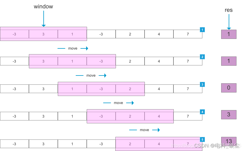
【Python/Pytorch 】-- 滑动窗口算法
文章目录 文章目录 00 写在前面01 基于Python版本的滑动窗口代码02 算法效果 00 写在前面 写这个算法原因是:训练了一个时序网络,该网络模型的时序维度为32,而测试数据的时序维度为90。因此需要采用滑动窗口的方法,生成一系列32…...

Clickhouse集群create drop database可删除集群数据库或只删除本地数据库
集群环境下,在任意一个节点创建数据库,如果加上了ON CLUSTER clustername,则在集群环境的所有节点上都创建了该数据库,并在集群环境的所有节点上都创建了该数据库对应的目录,且数据库的metadata_path对应的目录路径在所…...

【docker】adoptopenjdk/openjdk8-openj9:alpine-slim了解
adoptopenjdk/openjdk8-openj9:alpine-slim 是一个 Docker 镜像的标签,它指的是一个特定的软件包,用于在容器化环境中运行 Java 应用程序。 镜像相关的网站和资源: AdoptOpenJDK 官方网站 - AdoptOpenJDK 这是 AdoptOpenJDK 项目的官方网站&…...

Vscode interaction window
python 代码关联到 jupyter 模式 在代码前添加: # %%print("hellow wolrd!") 参考文档链接: https://code.visualstudio.com/docs/python/jupyter-support-py...
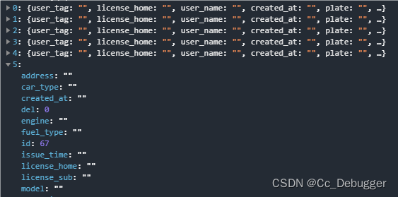
后端数据null前端统一显示成空
handleNullValues方法在封装请求接口返回数据时统一处理 // null 转 function handleNullValues(data) {// 使用递归处理多层嵌套的对象或数组function processItem(item) {if (Array.isArray(item)) {return item.map(processItem);} else if (typeof item object &&…...
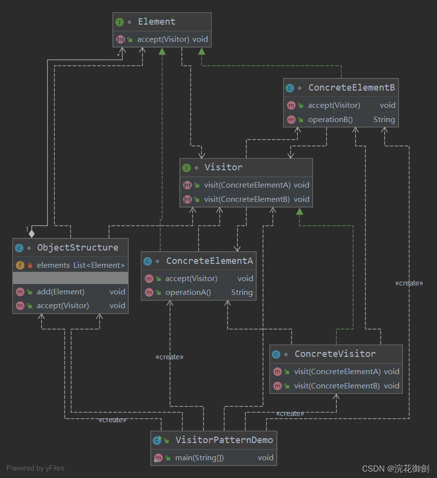
【设计模式深度剖析】【9】【行为型】【访问者模式】| 以博物馆的导览员为例加深理解
👈️上一篇:备忘录模式 | 下一篇:状态模式👉️ 设计模式-专栏👈️ 文章目录 访问者模式定义英文原话直译如何理解呢? 访问者模式的角色类图代码示例 访问者模式的应用优点缺点使用场景 示例解析:博物馆的导览员代码示例 访问…...
Salesforce‘s 爱因斯坦机器人助手引领工业聊天机器人时代
CRM的对话式人工智能助手,根据公司数据提供可靠的人工智能响应及日本工业聊天机器人现状 【前言】 爱因斯坦助手(Einstein Copilot)提供可靠的响应,因为它基于公司独特的数据和元数据,使其能够深入了解公司的业务和客…...

Day7—zookeeper基本操作
ZooKeeper介绍 ZooKeeper(动物园管理员)是一个分布式的、开源的分布式应用程序的协调服务框架,简称zk。ZooKeeper是Apache Hadoop 项目下的一个子项目,是一个树形目录服务。 ZooKeeper的主要功能 配置管理 分布式锁 集群管理…...
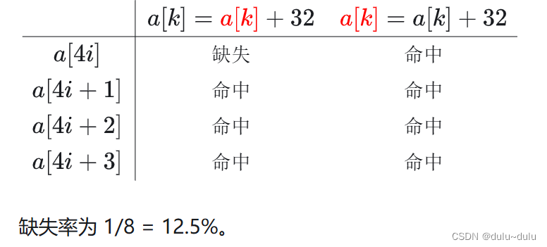
计算机组成原理---Cache的基本工作原理习题
对应知识点: Cache的基本原理 1.某存储系统中,主存容量是Cache容量的4096倍,Cache 被分为 64 个块,当主存地址和Cache地址采用直接映射方式时,地址映射表的大小应为()(假设不考虑一致维护和替…...
带来的适配问题:typeHandler)
springboot项目中切数据库(mysql-> pg)带来的适配问题:typeHandler
一、数据表中有一张表,名为role_permission,DDL如下: CREATE TABLE "public"."role_permission" ( "role_id" varchar(64) COLLATE "pg_catalog"."default" NOT NULL, "permiss…...

从零开始的<vue2项目脚手架>搭建:vite+vue2+eslint
前言 为了写 demo 或者研究某些问题,我经常需要新建空项目。每次搭建项目都要从头配置,很麻烦。所以我决定自己搭建一个项目初始化的脚手架(取名为 lily-cli)。 脚手架(scaffolding):创建项目时…...
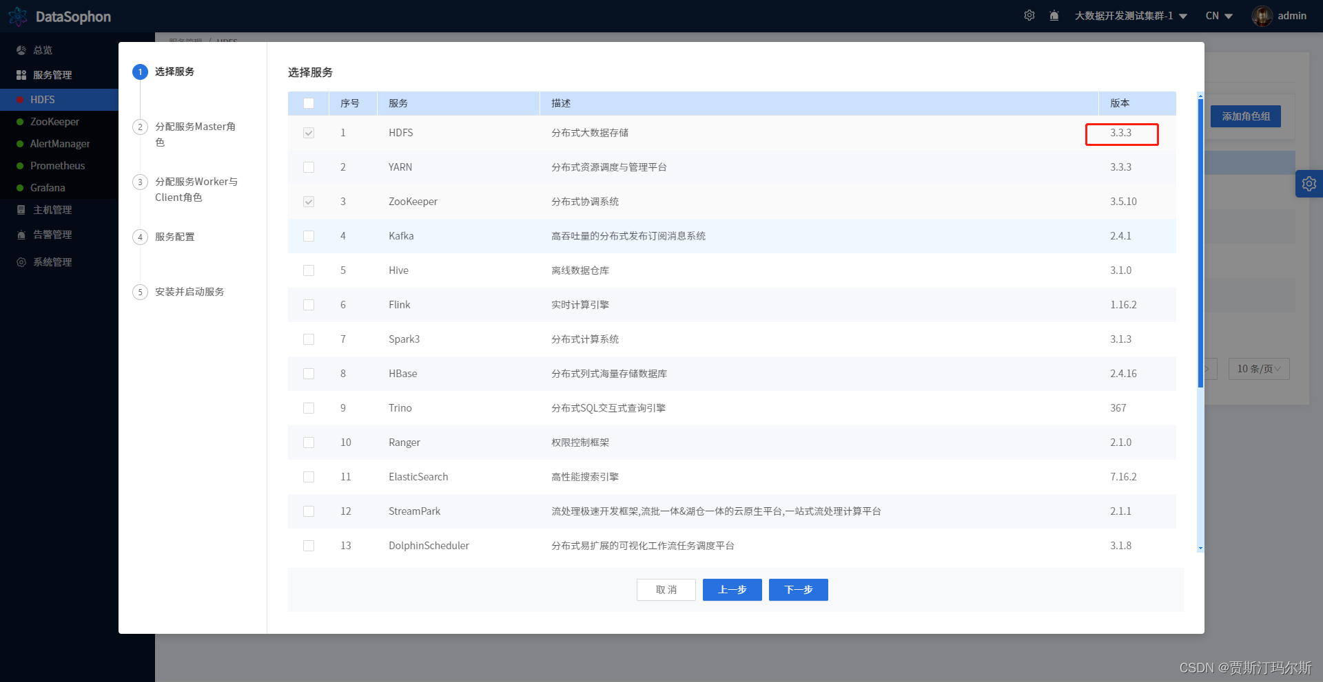
Hadoop升级失败,File system image contains an old layout version -64
原始版本 Hadoop 3.1.3 升级版本 Hadoop 3.3.3 报错内容如下 datasophon 部署Hadoop版本 查看Hadoop格式化版本 which hadoop-daemon.sh/bigdata/app/hadoop-3.1.3/sbin/hadoop-daemon.sh删除原来的旧版本 rm -rf /bigdata/app/hadoop-3.1.3查看环境变量 env|grep HADOOPHAD…...
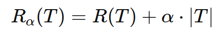
[机器学习算法]决策树
1. 理解决策树的基本概念 决策树是一种监督学习算法,可以用于分类和回归任务。决策树通过一系列规则将数据划分为不同的类别或值。树的每个节点表示一个特征,节点之间的分支表示特征的可能取值,叶节点表示分类或回归结果。 2. 决策树的构建…...
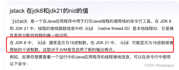
springboot应用cpu飙升的原因排除
1、通过top或者jps命令查到是那个java进程, top可以看全局那个进程耗cpu,而jps则默认是java最耗cpu的,比如找到进程是196 1.1 top (推荐)或者jps命令均可 2、根据第一步获取的进程号,查询进程里那个线程最占用cpu,发…...
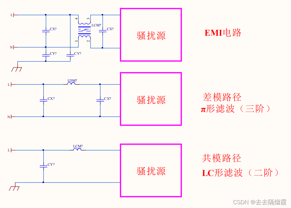
反激开关电源EMI电路选型及计算
EMI :开关电源对电网或者其他电子产品的干扰 EMI :传导与辐射 共模电感的滤波电路,La和Lb就是共模电感线圈。这两个线圈绕在同一铁芯上,匝数和相位都相 同(绕制反向)。 这样,当电路中的正常电流(差模&…...
vue3前端对接后端的图片验证码
vue3前端对接后端的图片验证码 <template> <image :src"captchaUrl" alt"图片验证码" click"refreshCaptcha"></image> </template><script setup>import {ref} from "vue";import {useCounterStore} …...
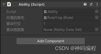
【Unity】RPG2D龙城纷争(四)要诀、要诀数据集
更新日期:2024年6月20日。 项目源码:第五章发布(正式开始游戏逻辑的章节) 索引 简介要诀数据集(AbilityDataSet)一、定义要诀数据集类二、要诀属性1.要诀类型2.攻击距离3.基础命中、暴击率4.基础属性加成5.…...
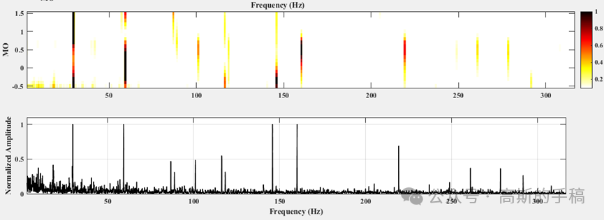
一种基于非线性滤波过程的旋转机械故障诊断方法(MATLAB)
在众多的旋转机械故障诊断方法中,包络分析,又称为共振解调技术,是目前应用最为成功的方法之一。首先,对激励引起的共振频带进行带通滤波,然后对滤波信号进行包络谱分析,通过识别包络谱中的故障相关的特征频…...

挑战杯推荐项目
“人工智能”创意赛 - 智能艺术创作助手:借助大模型技术,开发能根据用户输入的主题、风格等要求,生成绘画、音乐、文学作品等多种形式艺术创作灵感或初稿的应用,帮助艺术家和创意爱好者激发创意、提高创作效率。 - 个性化梦境…...
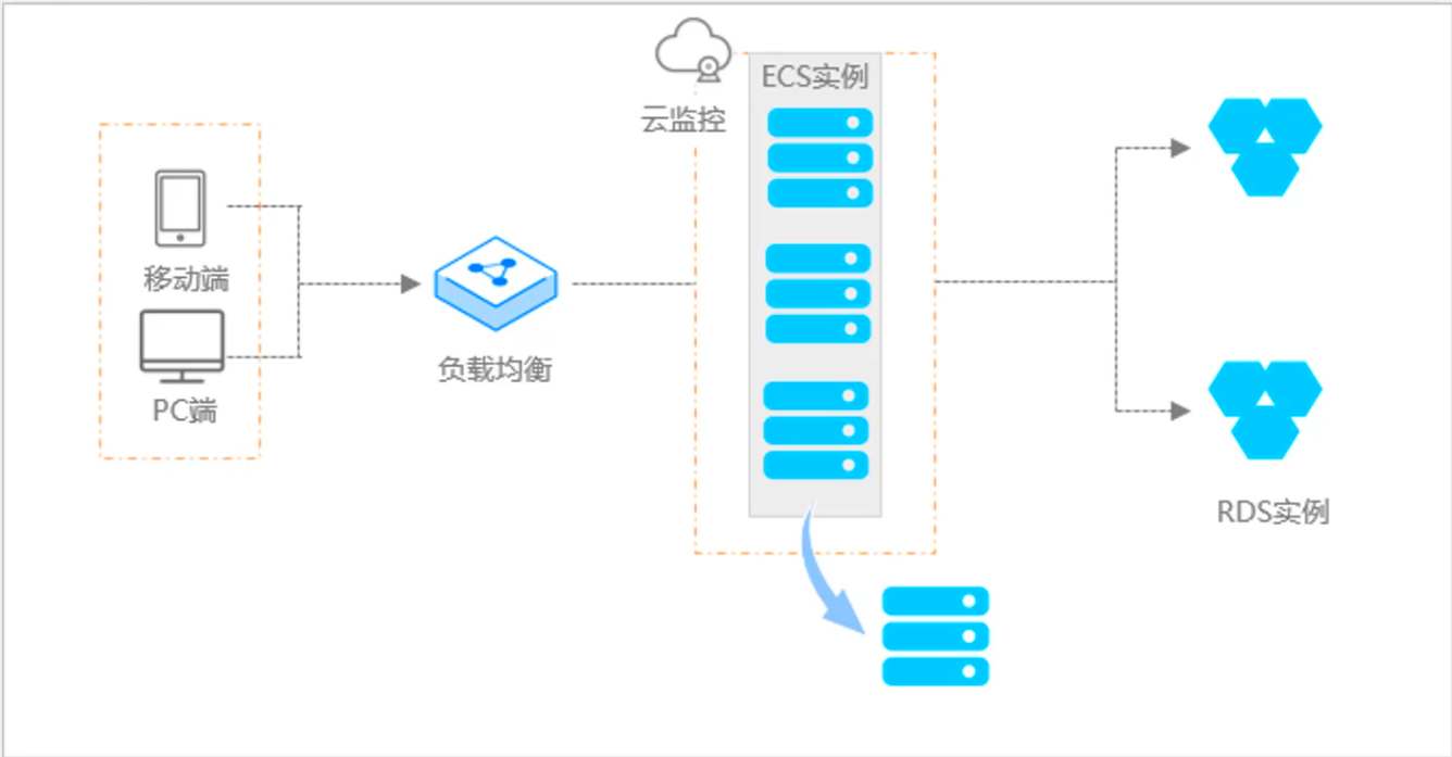
阿里云ACP云计算备考笔记 (5)——弹性伸缩
目录 第一章 概述 第二章 弹性伸缩简介 1、弹性伸缩 2、垂直伸缩 3、优势 4、应用场景 ① 无规律的业务量波动 ② 有规律的业务量波动 ③ 无明显业务量波动 ④ 混合型业务 ⑤ 消息通知 ⑥ 生命周期挂钩 ⑦ 自定义方式 ⑧ 滚的升级 5、使用限制 第三章 主要定义 …...
循环冗余码校验CRC码 算法步骤+详细实例计算
通信过程:(白话解释) 我们将原始待发送的消息称为 M M M,依据发送接收消息双方约定的生成多项式 G ( x ) G(x) G(x)(意思就是 G ( x ) G(x) G(x) 是已知的)࿰…...

深入理解JavaScript设计模式之单例模式
目录 什么是单例模式为什么需要单例模式常见应用场景包括 单例模式实现透明单例模式实现不透明单例模式用代理实现单例模式javaScript中的单例模式使用命名空间使用闭包封装私有变量 惰性单例通用的惰性单例 结语 什么是单例模式 单例模式(Singleton Pattern&#…...

laravel8+vue3.0+element-plus搭建方法
创建 laravel8 项目 composer create-project --prefer-dist laravel/laravel laravel8 8.* 安装 laravel/ui composer require laravel/ui 修改 package.json 文件 "devDependencies": {"vue/compiler-sfc": "^3.0.7","axios": …...

莫兰迪高级灰总结计划简约商务通用PPT模版
莫兰迪高级灰总结计划简约商务通用PPT模版,莫兰迪调色板清新简约工作汇报PPT模版,莫兰迪时尚风极简设计PPT模版,大学生毕业论文答辩PPT模版,莫兰迪配色总结计划简约商务通用PPT模版,莫兰迪商务汇报PPT模版,…...
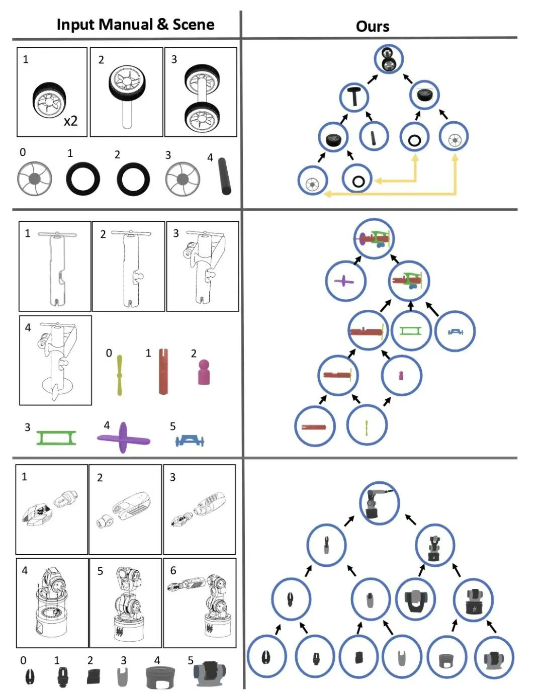
RSS 2025|从说明书学习复杂机器人操作任务:NUS邵林团队提出全新机器人装配技能学习框架Manual2Skill
视觉语言模型(Vision-Language Models, VLMs),为真实环境中的机器人操作任务提供了极具潜力的解决方案。 尽管 VLMs 取得了显著进展,机器人仍难以胜任复杂的长时程任务(如家具装配),主要受限于人…...
 + 力扣解决)
LRU 缓存机制详解与实现(Java版) + 力扣解决
📌 LRU 缓存机制详解与实现(Java版) 一、📖 问题背景 在日常开发中,我们经常会使用 缓存(Cache) 来提升性能。但由于内存有限,缓存不可能无限增长,于是需要策略决定&am…...
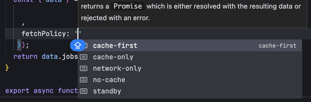
GraphQL 实战篇:Apollo Client 配置与缓存
GraphQL 实战篇:Apollo Client 配置与缓存 上一篇:GraphQL 入门篇:基础查询语法 依旧和上一篇的笔记一样,主实操,没啥过多的细节讲解,代码具体在: https://github.com/GoldenaArcher/graphql…...
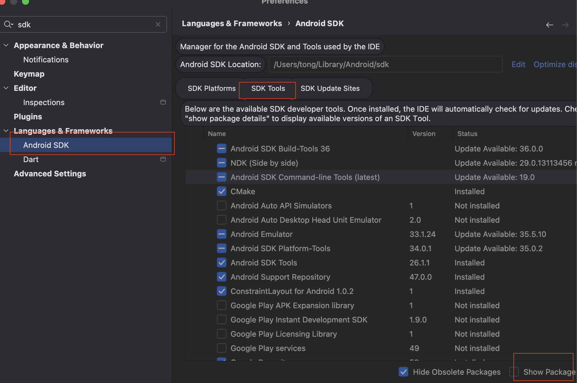
Mac flutter环境搭建
一、下载flutter sdk 制作 Android 应用 | Flutter 中文文档 - Flutter 中文开发者网站 - Flutter 1、查看mac电脑处理器选择sdk 2、解压 unzip ~/Downloads/flutter_macos_arm64_3.32.2-stable.zip \ -d ~/development/ 3、添加环境变量 命令行打开配置环境变量文件 ope…...