小波与傅里叶变换的对比(Python)
直接上代码,理论可以去知乎看。
#Import necessary libraries
%matplotlib inline
import numpy as np
import matplotlib.pyplot as plt
import seaborn as snsimport pywt
from scipy.ndimage import gaussian_filter1d
from scipy.signal import chirp
import matplotlib.gridspec as gridspec
from scipy import signal
from skimage import filters,img_as_float
from skimage.io import imread, imshow
from skimage.color import rgb2hsv, rgb2gray, rgb2yuv
from skimage import color, exposure, transform
from skimage.exposure import equalize_hist
from scipy import fftpack, ndimage
How to choose scale for wavelet transform
t_min=0
t_max=10
fs=100
dt = 1/fs
time = np.linspace(t_min, t_max, 1500)
#To understand the behaviour of scale, we used a smooth constant signal with a discontinuity. Adding discontinuity to the constant will have a rectangular shape.
w = chirp(time, f0=10, f1=50, t1=10, method='quadratic')#Compute Wavelet Transform
scale = [10,20,30,50,100]#Plot signal, FFT, and scalogram(to represent wavelet transform)
fig,axes =  plt.subplots(nrows=1,ncols=5,figsize=(25,4))
for i in range(2):for j in range(5):#Scalogramscales = np.arange(1,scale[j],1)coef,freqs = pywt.cwt(w,scales,'morl')freqs = pywt.scale2frequency('morl',scales,precision=8)if i == 0:axes[j].set_title("Scalogram from scale {} to {}".format(1,scale[j]))if i == 0:axes[j].pcolormesh(time, scales, coef,cmap='Greys')axes[j].set_ylabel("Scale")
plt.show();
scales = np.arange(1,20,1)
coef,freqs = pywt.cwt(w,scales,'morl',1/fs)
fig,axes =  plt.subplots(nrows=1,ncols=2,figsize=(12,5))
axes[0].set_title("Scalogram")
axes[0].pcolormesh(time, scales, coef,cmap='Greys')
axes[0].set_xlabel("Time")
axes[0].set_ylabel("Scale")
axes[1].set_title("Spectrogram")
axes[1].pcolormesh(time, freqs, coef,cmap='Greys')
axes[1].set_xlabel("Time")
axes[1].set_ylabel("Pseudo Frequency")
plt.show();
families = ['gaus1','gaus2','gaus3','gaus4','gaus5','gaus6','gaus7','gaus8','mexh','morl']
cols = 5
rows = 4
scales = np.arange(1,20,1)
fig,axes =  plt.subplots(nrows = rows,ncols=5,figsize=(3*cols,2*rows))
fig.tight_layout(pad=1.0, w_pad=1.0, h_pad=3)
for i,family in enumerate(families):c = i%5r = round(i//5)coef,freqs = pywt.cwt(w,scales,family,1/fs)psi, x = pywt.ContinuousWavelet(family).wavefun(level=10)axes[r*2,c].set_title(family)axes[(r*2)+1,c].pcolormesh(time, freqs, coef,cmap='Blues')axes[(r*2)+1,c].set_xlabel("Time")axes[(r*2)+1,c].set_ylabel("Scale")axes[r*2,c].plot(x, psi)axes[r*2,c].set_xlabel("X")axes[r*2,c].set_ylabel("Psi")
Constant Signal
fs = 100 #Sampling frequency
time = np.arange(-3,3,1/fs) #create time
n = len(time)
T=1/fs
print("We consider {} samples".format(n))
constant = np.ones(n) #Amblitude will be one(constant value)
freq =  np.linspace(-1.0/(2.0*T), 1.0/(2.0*T), n)#Compute Fourier transform of Constant signal
fft = fftpack.fft(constant)
freq = fftpack.fftfreq(time.shape[0],T)
phase  = np.angle(fft)
phase  = phase / np.pi#Compute Wavelet Transform
scales = np.arange(1,6,1)
coef,freqs = pywt.cwt(constant,scales,'gaus1')#Plot signal, FFT, and scalogram(to represent wavelet transform)
fig,axes =  plt.subplots(ncols=3,figsize=(18,4))#Signal
axes[0].set_title("Constant")
axes[0].plot(time, constant)
axes[0].set_xlabel("Time")
axes[0].set_ylabel("Amplitude")#Fourier
axes[1].set_title("Fourier Transform")
axes[1].plot(freq, np.abs(fft)/n)
axes[1].set_xlabel("Frequency")
axes[1].set_ylabel("Magnitude")#Scalogram
axes[2].set_title("Scalogram")
axes[2].pcolormesh(time, scales, coef,cmap='bone')
axes[2].set_xlabel("Time")
axes[2].set_ylabel("Scale")
plt.show();
Adding discontinuity to constant signal
constant[300:340]=0#Compute Fourier transform of Constant signal
fft = fftpack.fft(constant)
phase  = np.angle(fft)
phase  = phase / np.pi#Compute Wavelet Transform
scales = np.arange(1,6,1)
coef,freqs = pywt.cwt(constant,scales,'gaus1')#Plot signal, FFT, and scalogram(to represent wavelet transform)
fig,axes =  plt.subplots(ncols=3,figsize=(18,4))#Signal
axes[0].set_title("Constant")
axes[0].plot(time, constant)
axes[0].set_xlabel("Time")
axes[0].set_ylabel("Amplitude")#Fourier
axes[1].set_title("Fourier Transform")
axes[1].plot(freq, np.abs(fft)/n)
axes[1].set_xlabel("Frequency")
axes[1].set_ylabel("Magnitude")#Scalogram
axes[2].set_title("Scalogram")
axes[2].pcolormesh(time, scales, coef,cmap='bone')
axes[2].set_xlabel("Time")
axes[2].set_ylabel("Scale")
plt.show();
Rectangular Pulse
N = 50000 #number of samples
fs = 1000 #sample frequency
T = 1/fs #interval
time = np.linspace(-(N*T), N*T, N)
rect = np.zeros(time.shape)
for i in range(time.shape[0]):if time[i] > -0.5 and time[i] < 0.5:rect[i] = 1.0
print("We consider {} samples".format(N))
freq =  np.linspace(-1.0/(2.0*T), 1.0/(2.0*T), N)#compute Fourier Trainsform
fft_rect = np.fft.fft(rect)
fr = np.fft.fftfreq(N)
phase  = np.angle(fft_rect)
phase  = phase / np.pi
freqrect = np.fft.fftfreq(time.shape[-1])
fft_rect = np.fft.fftshift(fft_rect)#compute wavelet transform
scales = np.arange(1,25,1)
coef,freqs = pywt.cwt(rect,scales,'gaus1')#Plot
#signal
fig,axes =  plt.subplots(ncols=3,figsize=(21,5))
axes[0].set_title("Rectangular signal")
axes[0].plot(time, rect)
axes[0].set_xlim(-1,1)
axes[0].set_xlabel("Time")
axes[0].set_ylabel("rectangular pulse")#Fourier transform
axes[1].set_title("Fourier Transform")
axes[1].plot(freq,np.abs(fft_rect)*2/fs)
axes[1].set_xlim(-40,40)
axes[1].set_xlabel("Frequency")
axes[1].set_ylabel("Magnitude")#wavelet
axes[2].set_title("Scalogram ")
axes[2].pcolormesh(time, scales, coef,cmap='bone')
axes[2].set_xlim(-2,2)
axes[2].set_xlabel("Time")
axes[2].set_ylabel("Scale")
plt.show();
Sine and cosine waves
fs = 1000 #sampling frequency
interval = 1/fs #sampling interval
t_min = -1 #start time
t_max = 1 # end time
dt=1/fs
time = np.arange(t_min,t_max,interval)n = len(time)
print("We consider {} samples".format(n))f = (fs/2)*np.linspace(0,1,int(n/2)) #frequencyfreq = [200,130] #signal frequencies
scales1 = np.arange(1,20,1)#Create signal with 200 hz frequency
sinewave1 = np.sin(2*np.pi*freq[0]*time)
new = sinewave1/np.square(time)
#compute fourier transform
fft1 = np.fft.fft(sinewave1)
fr = np.fft.fftfreq(n, d=dt)
phase  = np.angle(fft1)
phase  = phase / np.pi
fft1 = fft1[0:int(n/2)]#compute wavelet
coef1,freqs1 = pywt.cwt(sinewave1,scales1,'morl')#plot
gs = gridspec.GridSpec(2,2)
gs.update(left=0, right=4,top=2,bottom=0, hspace=.2,wspace=.1)
ax = plt.subplot(gs[0, :])
ax.set_title("Sinusoidal Signal - 200 Hz")
ax.plot(time,sinewave1)
ax.set_xlabel("Time(s)")
ax.set_ylabel("Amplitude")
ax2 = plt.subplot(gs[1, 0])
ax2.plot(f,np.abs(fft1)*2/fs)
ax2.set_xlabel("Frequency")
ax2.set_ylabel("DFT values")
ax3 = plt.subplot(gs[1, 1])
ax3.pcolormesh(time, freqs1/dt, coef1)
ax3.set_xlabel("Time")
ax3.set_ylabel("Frequency")
plt.show;
scales = np.arange(1,20,1)
#Create signal with 130 hz frequency
sinewave2 = np.sin(2*np.pi*freq[1]*time)#compute fourier transform
fft2 = np.fft.fft(sinewave2)
fft2=fft2[0:int(n/2)]#compute wavelet
coef2,freqs2 = pywt.cwt(sinewave2,scales,'morl')
#plot
gs = gridspec.GridSpec(2,2)
gs.update(left=0, right=4,top=2,bottom=0, hspace=.2,wspace=.1)
ax = plt.subplot(gs[0, :])
ax.set_title("Sinusoidal Signal - 130 Hz")
ax.plot(time,sinewave2)
ax.set_xlabel("Time(s)")
ax.set_ylabel("Amplitude")
ax2 = plt.subplot(gs[1, 0])
ax2.plot(f,np.abs(fft2)*2/fs)
ax2.set_xlim(0,300)
ax2.set_xlabel("Frequency")
ax2.set_ylabel("Magnitude")
ax3 = plt.subplot(gs[1, 1])
ax3.pcolormesh(time, freqs2/dt, coef2)
ax3.set_xlabel("Time")
ax3.set_ylabel("Scale")
plt.show();
scales = np.arange(1,30,1)sum = sinewave1+sinewave2
fft3 = np.fft.fft(sum)
fft3=fft3[0:int(n/2)]
coef3,freqs3 = pywt.cwt(sum,scales,'morl')#plot
gs = gridspec.GridSpec(2,2)
gs.update(left=0, right=4,top=2,bottom=0, hspace=.2,wspace=.1)ax = plt.subplot(gs[0, :])
ax.set_title("Sum of Sinusoidal")
ax.plot(time,sum)
ax.set_xlabel("Time(s)")
ax.set_ylabel("Amplitude")
ax2 = plt.subplot(gs[1, 0])
ax2.plot(f,np.abs(fft3)*2/fs)
ax2.set_xlabel("Frequency")
ax2.set_ylabel("Magnitude")
ax3 = plt.subplot(gs[1, 1])
ax3.pcolormesh(time, freqs3/dt, coef3)
ax3.set_xlabel("Time")
ax3.set_ylabel("Frequency")
plt.show();
Non stationary signals
size = len(time)//3
scales = np.arange(1,31,1)
sig = np.zeros(time.shape)
sig[:size]=np.sin(2*np.pi*200*time[:size])
sig[size:size*2]=np.sin(2*np.pi*130*time[size:size*2])
sig[size*2:]=np.cos(2*np.pi*50*time[size*2:])
fft = np.fft.fft(sig)
fft=fft[0:int(n/2)]
coef,freqs = pywt.cwt(sig,scales,'gaus8')
stft_f, stft_t, Sxx = signal.spectrogram(sig, fs,window='hann', nperseg=64)
#plot
gs = gridspec.GridSpec(2,2)
gs.update(left=0, right=4,top=2,bottom=0, hspace=.2,wspace=.1)ax = plt.subplot(gs[0, 0])
ax.set_title("Sinusoidal Signal- Frequency vary over time")
ax.plot(time,sig)
ax.set_xlabel("Time(s)")
ax.set_ylabel("Amplitude")
ax1 = plt.subplot(gs[0, 1])
ax1.plot(f,np.abs(fft)*2/fs)
ax1.set_xlabel("Frequency")
ax1.set_ylabel("Magnitude")
ax2 = plt.subplot(gs[1, 0])
ax2.pcolormesh(stft_t, stft_f, Sxx)
ax2.set_ylabel("Frequency")
ax3 = plt.subplot(gs[1, 1])
ax3.pcolormesh(time, freqs/dt, coef)
ax3.set_xlabel("Time")
ax3.set_ylabel("Frequency")
Linear Chirp Signal
def plot_chirp_transforms(type_,f0,f1):#Create linear chirp signal with frequency between 50Hz and 10Hzt_min=0t_max=10time = np.linspace(t_min, t_max, 1500)N = len(time)interval = (t_min+t_max)/Nfs = int(1/interval)dt=1/fsf = (fs/2)*np.linspace(0,1,int(N/2))w1 = chirp(time, f0=f0, f1=f1, t1=10, method=type_.lower())#Compute FFTw1fft = np.fft.fft(w1)w1fft=w1fft[0:int(N/2)]#Compute Wavelet transformscales=np.arange(1,50,1)wcoef,wfreqs = pywt.cwt(w1,scales,'morl')#Compute Short Time Fourier transfomrstft_f, stft_t, Sxx = signal.spectrogram(w1, fs,window='hann', nperseg=64,noverlap=32)#Plot the resultsgs = gridspec.GridSpec(2,2)gs.update(left=0, right=4,top=2,bottom=0, hspace=.2,wspace=.1)ax = plt.subplot(gs[0, 0])ax.set_title("Chirp - "+type_+" ({}Hz to {}Hz)".format(f0,f1))ax.plot(time,w1)ax.set_xlabel("Time(s)")ax.set_ylabel("Amplitude")ax1 = plt.subplot(gs[0, 1])ax1.plot(f,np.abs(w1fft)*2/fs)plt.grid()ax1.set_title("FFT - "+type_+" chirp signal ({}Hz to {}Hz)".format(f0,f1))ax1.set_xlabel("Frequency")ax1.set_ylabel("Magnitude")ax2 = plt.subplot(gs[1, 0])ax2.set_title("STFT - "+type_+" chirp signal ({}Hz to {}Hz)".format(f0,f1))ax2.pcolor(stft_t, stft_f, Sxx,cmap='copper')ax2.set_xlabel("Time")ax2.set_ylabel("Frequency")ax3 = plt.subplot(gs[1, 1])ax3.set_title("WT - "+type_+" chirp signal ({}Hz to {}Hz)".format(f0,f1))ax3.pcolor(time, wfreqs/dt, wcoef,cmap='copper')ax3.set_ylim(5,75)ax3.set_xlabel("Time")ax3.set_ylabel("Frequency")
plot_chirp_transforms('Linear',50,10)
plot_chirp_transforms('Linear',10,50)
plot_chirp_transforms('Quadratic',50,10)
Trapezoid
N = 5000 #number of samples
fs = 1000 #sample frequency
T = 1/fs #interval
time = np.linspace(-5, 5, N)
trapzoid_signal = (time*np.where(time>0,1,0))-((time-1)*np.where((time-1)>0,1,0))-((time-2)*np.where((time-2)>0,1,0))+((time-3)*np.where((time-3)>0,1,0))#tra = trapzoid_signal(time)scales = np.arange(1,51,1)
coef,freqs = pywt.cwt(trapzoid_signal,scales,'gaus1')
#compute Fourier Trainsform
fft = np.fft.fft(trapzoid_signal)
freq = np.fft.fftfreq(time.shape[-1],T)
fftShift = np.fft.fftshift(fft)
freqShift=np.fft.fftshift(freq)#Plot signal and FFT
fig,axes =  plt.subplots(nrows=2,ncols=3,figsize=(24,10))
axes[0,0].set_title("Trapezoidal signal")
axes[0,0].plot(time, trapzoid_signal)
axes[0,0].set_xlabel("Time")
axes[0,0].set_ylabel("Trapezoidal pulse")
axes[0,1].set_title("Fourier Transform - trapezoidal")
axes[0,1].plot(freqShift,np.abs(fftShift)*2/fs)
axes[0,1].set_xlim(-20,20)
axes[0,1].set_xlabel("Frequency")
axes[0,1].set_ylabel("Magnitude")
axes[0,2].set_title("Scalogram - trapezoidal")
axes[0,2].pcolor(time,scales,coef,cmap='BrBG')
axes[0,2].set_xlim(-5,5)
axes[0,2].set_xlabel("Time")
axes[0,2].set_ylabel("Scale")trapzoid_signal = ((time+1)*np.where((time+1)>0,1,0))-(time*np.where(time>0,1,0))-((time-1)*np.where((time-1)>0,1,0))+((time-2)*np.where((time-2)>0,1,0))
coef,freqs = pywt.cwt(trapzoid_signal,scales,'gaus1')
#compute Fourier Trainsform
fft = np.fft.fft(trapzoid_signal)
freq = np.fft.fftfreq(time.shape[-1],T)
fftShift = np.fft.fftshift(fft)
freqShift=np.fft.fftshift(freq)#Plot signal and FFT
axes[1,0].plot(time, trapzoid_signal)
axes[1,0].set_xlabel("Time")
axes[1,0].set_ylabel("Trapezoidal pulse")
axes[1,1].plot(freqShift,np.abs(fftShift)*2/fs)
axes[1,1].set_xlim(-20,20)
axes[1,1].set_xlabel("Frequency")
axes[1,1].set_ylabel("Magnitude")
axes[1,2].pcolor(time,scales,coef,cmap='BrBG')
axes[1,2].set_xlim(-5,5)
axes[1,2].set_xlabel("Time")
axes[1,2].set_ylabel("Scale")
#Image Generation
sigma = 20
fake_image = np.repeat(a=np.repeat(a=160,repeats=512),repeats=512).reshape([512,512])
fake_image_translated = fake_image.copy()
fake_image[250:350,200:300] = 190
fake_image_translated[250:350,250:350] = 190
fake_image = filters.gaussian(fake_image, sigma=sigma, preserve_range=True)
fake_image_translated = filters.gaussian(fake_image_translated, sigma=sigma, preserve_range=True)
fake_image = rgb2gray(fake_image)/255
fake_image_translated = rgb2gray(fake_image_translated)/255#Fourier transform
fft_fake = fftpack.fft2(fake_image)
fft_fake = fftpack.fftshift(fft_fake)
fft_fake2 = fftpack.fft2(fake_image_translated)
fft_fake2 = fftpack.fftshift(fft_fake2)#Plot
fig,axes = plt.subplots(ncols=4,figsize=(16,4));
axes[0].set_title("Fake Image");
axes[0].imshow(fake_image,cmap='gray');
axes[1].set_title("FFT");
axes[1].imshow(np.log(np.abs(fft_fake)),cmap='gray');
axes[2].set_title("Shifted Image");
axes[2].imshow(fake_image_translated,cmap='gray');
axes[3].set_title("FFT-shifted image");
axes[3].imshow(np.log(np.abs(fft_fake2)),cmap='gray');
plt.show();
titles = ['Approximation', ' Horizontal detail','Vertical detail', 'Diagonal detail']
coeffs_fi = pywt.dwt2(fake_image, 'haar')
coeffs_fi_translated = pywt.dwt2(fake_image_translated, 'haar')
coef_array = []
cA1, (cH1, cV1, cD1) = coeffs_fi
cA2, (cH2, cV2, cD2) = coeffs_fi_translated
coef_array.append([cA1,cH1, cV1, cD1])
coef_array.append([cA2,cH2, cV2, cD2])
fig,axes = plt.subplots(nrows=2,ncols=5,figsize=(25,10))
axes[0,0].set_title("Image")
axes[0,0].imshow(fake_image,cmap='gray')
axes[1,0].set_title("Image")
axes[1,0].imshow(fake_image_translated,cmap='gray')
for i,arr in enumerate(coef_array):for idx,coef in enumerate(arr):axes[i,idx+1].set_title(titles[idx])axes[i,idx+1].imshow(coef,cmap='gray')
from scipy import ndimage#Image Generation
line_image = np.repeat(a=np.repeat(a=0,repeats=512),repeats=512).reshape([512,512])
line_image_translated = line_image.copy()
line_image[192:320,128:354] = 165
line_image[224:288,192:320] = 70
line_image_translated[128:354,192:320] = 165
line_image_translated[192:320,224:288] = 70
line_image = filters.gaussian(line_image, sigma=sigma, preserve_range=True)
line_image_translated = filters.gaussian(line_image_translated, sigma=sigma, preserve_range=True)
line_image = rgb2gray(line_image)/255
line_image_translated = rgb2gray(line_image_translated)/255
line_image_rot = ndimage.rotate(line_image, 45, reshape=False)#Fourier transform
fft_line = fftpack.fft2(line_image)
fft_line = fftpack.fftshift(fft_line)
fft_line_t = fftpack.fft2(line_image_translated)
fft_line_t = fftpack.fftshift(fft_line_t)
fft_line_r = fftpack.fft2(line_image_rot)
fft_line_r = fftpack.fftshift(fft_line_r)#Plot
fig,axes = plt.subplots(ncols=6,figsize=(24,4))
axes[0].set_title("Fake Image")
axes[0].imshow(line_image,cmap='gray')
axes[1].set_title("FFT")
axes[1].imshow(np.log(np.abs(fft_line)),cmap='gray')
axes[2].set_title("Shifted Image")
axes[2].imshow(line_image_translated,cmap='gray')
axes[3].set_title("FFT-shifted image")
axes[3].imshow(np.log(np.abs(fft_line_t)),cmap='gray')
axes[4].set_title("Rotated image")
axes[4].imshow(line_image_rot,cmap='gray')
axes[5].set_title("FFT-Rotated")
axes[5].imshow(np.log(np.abs(fft_line_r)),cmap='gray')
plt.show();
coef_line = pywt.dwt2(line_image, 'haar')
coef_line_t = pywt.dwt2(line_image_translated, 'haar')
coef_line_r = pywt.dwt2(line_image_rot, 'haar')
dwt_coef_array = []
lcA1, (lcH1, lcV1, lcD1) = coef_line
lcA2, (lcH2, lcV2, lcD2) = coef_line_t
lcA3, (lcH3, lcV3, lcD3) = coef_line_r
dwt_coef_array.append([lcA1,lcH1, lcV1, lcD1])
dwt_coef_array.append([lcA2,lcH2, lcV2, lcD2])
dwt_coef_array.append([lcA3,lcH3, lcV3, lcD3])
fig,axes = plt.subplots(nrows=3,ncols=5,figsize=(25,15))
axes[0,0].set_title("Fake Image")
axes[0,0].imshow(line_image,cmap='gray')
axes[1,0].set_title("Translated Image")
axes[1,0].imshow(line_image_translated,cmap='gray')
axes[2,0].set_title("Rotated Image")
axes[2,0].imshow(line_image_rot,cmap='gray')
for i,arr in enumerate(dwt_coef_array):for idx,coef in enumerate(arr):axes[i,idx+1].set_title(titles[idx])axes[i,idx+1].imshow(coef,cmap='gray')
from PIL import Image
# open the original image
original_img = Image.open("/content/drive/MyDrive/DSIP/parrot1.jpg")#rotate image
rot_180 = original_img.rotate(180, Image.NEAREST, expand = 1)# close all our files objectI = np.array(original_img)
I_rot = np.array(rot_180)original_img.close()I_grey = rgb2gray(I)
I_rot_grey = rgb2gray(I_rot)fft2 = fftpack.fft2(I_grey)
fftshift = fftpack.fftshift(fft2)
fftrot2 = fftpack.fft2(I_rot_grey)
fftrotshift = fftpack.fftshift(fftrot2)coeffs2 = pywt.dwt2(I_grey, 'haar')
cA, (cH, cV, cD) = coeffs2
titles = ['Approximation', ' Horizontal detail','Vertical detail', 'Diagonal detail']
coeffs3 = pywt.dwt2(I_rot_grey, 'haar')
cA1, (cH1, cV1, cD1) = coeffs3
fig,axes = plt.subplots(ncols=6,nrows=2,figsize=(24,8))axes[0,0].set_title("Image")
axes[0,0].imshow(img_as_float(I_grey),cmap='gray')
axes[0,1].set_title("FFT")
axes[0,1].imshow(np.log(np.abs(fftshift)),cmap='gray')
axes[1,0].set_title("Flip Image")
axes[1,0].imshow(img_as_float(I_rot_grey),cmap='gray')
axes[1,1].set_title("FFT-flip image")
axes[1,1].imshow(np.log(np.abs(fftrotshift)),cmap='gray')for idx,coef in enumerate((cA,cH,cV,cD)):axes[0,idx+2].set_title(titles[idx])axes[0,idx+2].imshow(coef,cmap='gray')
for idx,coef in enumerate((cA1,cH1,cV1,cD1)):axes[1,idx+2].set_title(titles[idx])axes[1,idx+2].imshow(coef,cmap='gray')
plt.show();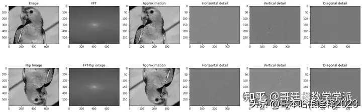
知乎学术咨询:
https://www.zhihu.com/consult/people/792359672131756032?isMe=1
擅长领域:现代信号处理,机器学习,深度学习,数字孪生,时间序列分析,设备缺陷检测、设备异常检测、设备智能故障诊断与健康管理PHM等。
相关文章:
小波与傅里叶变换的对比(Python)
直接上代码,理论可以去知乎看。 #Import necessary libraries %matplotlib inline import numpy as np import matplotlib.pyplot as plt import seaborn as snsimport pywt from scipy.ndimage import gaussian_filter1d from scipy.signal import chirp import m…...

Linux-sqlplus安装
1.下载安装包 下载入口:安装包 下载对应版本: oracle-instantclient-sqlplus-21.14.0.0.0-1.x86_64.rpm oracle-instantclient-basic-21.14.0.0.0-1.x86_64.rpm oracle-instantclient-devel-21.14.0.0.0-1.x86_64.rpm 2.安装 [rootpromethues-01 tmp…...

LeetCode 算法:课程表 c++
原题链接🔗:课程表 难度:中等⭐️⭐️ 题目 你这个学期必须选修 numCourses 门课程,记为 0 到 numCourses - 1 。 在选修某些课程之前需要一些先修课程。 先修课程按数组 prerequisites 给出,其中 prerequisites[i]…...

前端面试题30(闭包和作用域链的关系)
闭包和作用域链在JavaScript中是紧密相关的两个概念,理解它们之间的关系对于深入掌握JavaScript的执行机制至关重要。 作用域链 作用域链是一个链接列表,它包含了当前执行上下文的所有父级执行上下文的变量对象。每当函数被调用时,JavaScri…...
A股本周在3000点以下继续筑底,本周依然继续探底?
夜已深,市场传来了3个浓烈的消息,炸锅了,恐有大事发生,马上告诉所有人: 消息面: 1、中国经济周刊首席评论员钮文新称:不要等中小投资者都彻底希望,销户离场了,才发现该…...

Javadoc介绍
Javadoc 是用于生成 Java 代码文档的工具。它利用特定的注释格式,将 Java 源代码中的注释提取出来,并生成 HTML 文档。Javadoc 注释通常位于类、接口、构造函数、方法和字段的声明之前,以 /** 开始,以 */ 结束。以下是 Javadoc 注释的一些主要元素和使用方法: 基本语法 …...

C# Application.DoEvents()的作用
文章目录 1、详解 Application.DoEvents()2、示例处理用户事件响应系统事件控制台输出游戏和多媒体应用与操作系统的交互 3、注意事项总结 Application.DoEvents() 是 .NET 框架中的一个方法,它主要用于处理消息队列中的事件。在 Windows 应用程序中,当一…...
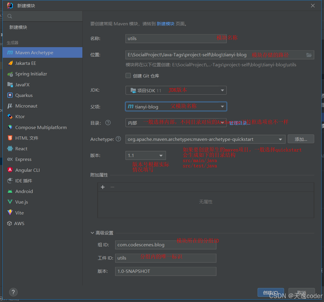
IDEA如何创建原生maven子模块
文件 -> 新建 -> 新模块 -> Maven ArcheTypeMaven ArcheType界面中的输入框介绍 名称:子模块的名称位置:子模块存放的路径名创建Git仓库:子模块不单独作为一个git仓库,无需勾选JDK:JDK版本号父项:…...

LCD EMC 辐射 测试随想
最近做几个产品过认证。 有带2.8寸 MCU8080接口的小屏(320 X 240),也有RGB接口的10.1寸的大屏(800*600). 以下为个人随想,不知道是否正确,仅作记录。 测试发现辐射的核心问题还是在于时钟及其倍频所产生的尖峰。 记得读…...

Docker安装遇到问题:curl: (7) Failed to connect to download.docker.com port 443: 拒绝连接
问题描述 首先,完全按照Docker官方文档进行安装: Install Docker Engine on Ubuntu | Docker Docs 在第1步:Set up Dockers apt repository,执行如下指令: sudo curl -fsSL https://download.docker.com/linux/ubu…...
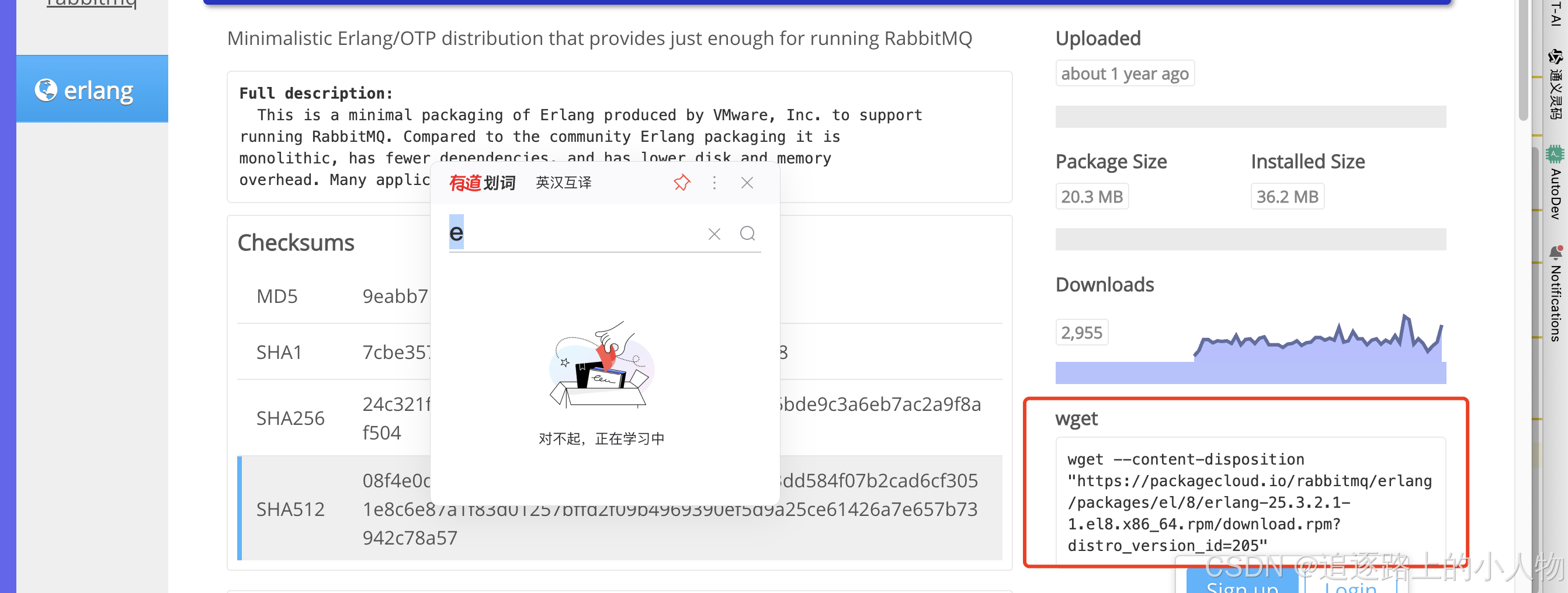
阿里云安装rabbitMQ
1、首先看linux 版本 uname -a如果时centos 7 可以参考其他文档。我这里是centos 8 这个很重要 。网上全是按centos7 按照。导致我前面一直安装不上 各种问题。 2、查看rabbitmq 对应 erl 的版本下载 https://www.rabbitmq.com/docs/which-erlang 选择rabbitmq 3.11.19 选择…...

中文大模型基准测评2024上半年报告
中文大模型基准测评2024上半年报告 原创 SuperCLUE CLUE中文语言理解测评基准 2024年07月09日 18:09 浙江 SuperCLUE团队 2024/07 背景 自2023年以来,AI大模型在全球范围内掀起了有史以来规模最大的人工智能浪潮。进入2024年,全球大模型竞争态势日益加…...

新火种AI|OpenAI的CEO又有新动作?这次他成立了AI健康公司
作者:一号 编辑:美美 AI技术即将改变医疗健康市场。 就在前两天,人工智能和医疗健康领域迎来了一个重要时刻。OpenAI的CEO萨姆阿尔特曼(Sam Altman)与Thrive Global的CEO阿里安娜赫芬顿(Arianna Huffing…...

中介子方程五十
XXFXXaXnXaXXαXLXyXXWXuXeXKXXiXyXΣXXΣXXVXuXhXXWXηXXiXhXXpXXhXiXXηXWXXhXuXVXXΣXXΣXyXiXXKXeXuXWXXyXLXαXXaXnXaXXFXXaXnXaXXαXLXyXXWXuXeXKXXiXyXΣXXΣXXVXuXhXXWXηXXiXhXXpXXhXiXXηXWXXhXuXVXXΣXXΣXyXiXXKXeXuXWXXyXLXαXXaXnXaXXFXXuXXWXXuXXdXXrXXαXXuXpX…...

如何借助社交媒体影响者的力量,让品牌影响力倍增?
一、引言:为何社交媒体影响者如此关键? 在信息爆炸的今天,社交媒体已成为塑造消费者行为与品牌认知的重要渠道。社交媒体影响者,凭借其在特定领域的专业知识、庞大的粉丝基础及高度的互动性,成为了品牌传播不可忽视的…...

Python面试题:Python 中的 `property` 函数有什么用?
在 Python 中,property 函数用于创建和管理类中的属性。它允许你将方法转换为属性,这样你可以像访问变量一样访问这些方法。这对于控制属性的访问和修改非常有用,因为它允许你在属性访问时执行额外的逻辑(如验证或计算)…...
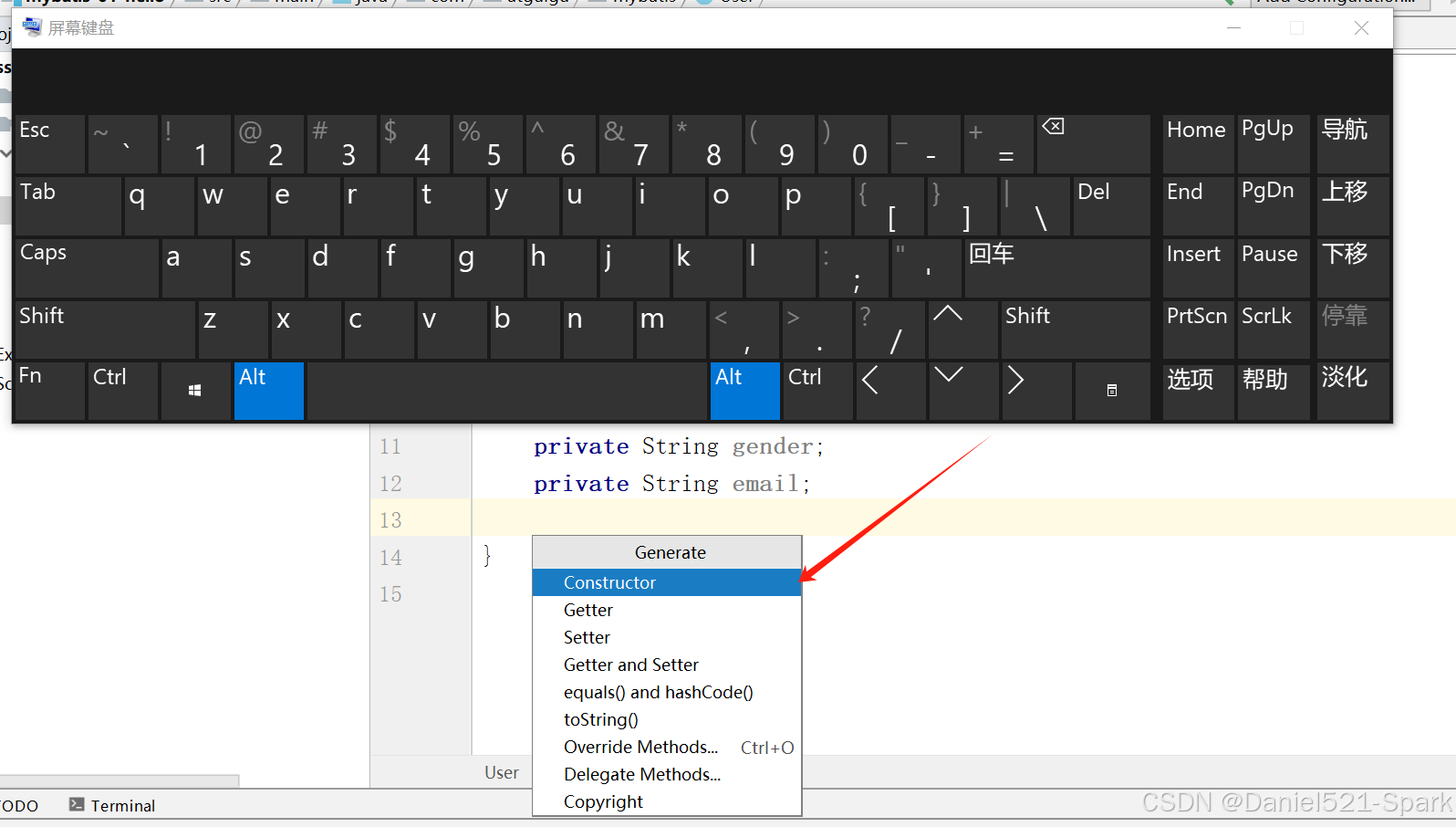
十五、小型电脑没有数字键及insert,怎么解决IDEA快速插入getset构造这些方法
🌻🌻目录 一、小型电脑没有数字键及insert,怎么解决IDEA快速插入getset构造这些方法 一、小型电脑没有数字键及insert,怎么解决IDEA快速插入getset构造这些方法 解决: 1.winR打开搜索 2.osk回车 屏幕就出现了这样的一…...

【鸿蒙学习笔记】属性学习迭代笔记
这里写目录标题 TextImageColumnRow Text Entry Component struct PracExample {build() {Row() {Text(文本描述).fontSize(40)// 字体大小.fontWeight(FontWeight.Bold)// 加粗.fontColor(Color.Blue)// 字体颜色.backgroundColor(Color.Red)// 背景颜色.width(50%)// 组件宽…...

工具推荐:滴答清单
官网地址:DIDA:Todo list, checklist and task manager app for Android, iPhone and Web 使用近一个月,特别方便,使用感受非常棒,功能全面。 我主要用了以下功能: 1、每日事项提醒:写作,背字…...
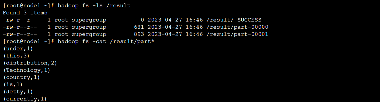
阶段三:项目开发---大数据开发运行环境搭建:任务4:安装配置Spark集群
任务描述 知识点:安装配置Spark 重 点: 安装配置Spark 难 点:无 内 容: Apache Spark 是专为大规模数据处理而设计的快速通用的计算引擎。Spark是UC Berkeley AMP lab (加州大学伯克利分校的AMP实验室)所开源的类Hadoop …...
)
UOS系统下WPS卸载不干净?手把手教你用命令行精准清理(附dpkg/apt组合拳)
UOS系统下WPS卸载不干净?手把手教你用命令行精准清理 在UOS系统日常使用中,WPS Office作为常用办公软件,有时因版本更新或功能调整需要彻底卸载。但不少用户发现,通过图形界面或简单命令卸载后,系统中仍残留配置文件、…...

Office RibbonX Editor:让Office界面定制变得像搭积木一样简单
Office RibbonX Editor:让Office界面定制变得像搭积木一样简单 【免费下载链接】office-ribbonx-editor An overhauled fork of the original Custom UI Editor for Microsoft Office, built with WPF 项目地址: https://gitcode.com/gh_mirrors/of/office-ribbon…...

从多路复用到三维光阵:Arduino驱动8x8x8 LED立方体全解析
1. 项目概述:用Arduino点亮一个三维世界几年前,我第一次在创客展上看到一个8x8x8的LED立方体,那种由数百个光点构成的、在三维空间中流动的动画效果,瞬间就把我吸引住了。它不像普通的平面LED屏,而是真正有“深度”的光…...

PentestGPT实战部署指南:AI驱动的渗透测试工作流落地
1. 这不是另一个“AI安全”的概念玩具,而是一套能真正跑起来的渗透测试辅助工作流“PentestGPT”这个名字刚在GitHub上出现时,我第一反应是点开又关掉——过去三年里,我见过太多打着“AI渗透”旗号的项目:有的只是把ChatGPT API封…...

FeHelper前端助手:30+开发工具集,让你的浏览器变身效率神器
FeHelper前端助手:30开发工具集,让你的浏览器变身效率神器 【免费下载链接】FeHelper 😍FeHelper--Web前端助手(Awesome!Chrome & Firefox & MS-Edge Extension, All in one Toolbox!) 项目地址:…...

从“DOC/PDF”到“WPS”:细看GJB438C-2021文档格式要求背后的国产化信号与落地指南
从“DOC/PDF”到“WPS”:GJB438C-2021文档格式变革的深度解读与实施策略 当一份国家军用标准在文档格式描述中刻意删除"DOC/PDF"字样,转而明确标注"(WPS)文档处理器"时,这绝非简单的技术参数调整。…...
)
从零到上机:我的第一个Quest 3空间锚点应用是如何跑起来的(附完整Unity工程)
从零到上机:我的第一个Quest 3空间锚点应用是如何跑起来的(附完整Unity工程)第一次戴上Meta Quest 3时,那种虚拟与现实交织的震撼感至今难忘。但作为开发者,更让我着迷的是如何让虚拟物体在真实空间中"记住"…...

CPU架构启发的智能仓储布局优化实践
1. 仓库布局优化的核心挑战与创新机遇在物流仓储领域,拣货环节通常占据运营成本的55%-65%,而其中约50%的时间消耗在无效行走路径上。传统矩形仓库布局虽然易于规划和施工,但其正交的通道设计导致拣货员需要频繁进行90度转向,这种&…...

Hindsight测试策略:单元测试、集成测试和端到端测试
Hindsight测试策略:单元测试、集成测试和端到端测试 【免费下载链接】hindsight Hindsight: Agent Memory That Learns 项目地址: https://gitcode.com/GitHub_Trending/hindsight2/hindsight Hindsight作为一款专注于Agent Memory的开源项目,其可…...

三步让小爱音箱秒变AI语音助手:MiGPT深度配置指南
三步让小爱音箱秒变AI语音助手:MiGPT深度配置指南 【免费下载链接】mi-gpt 🏠 将小爱音箱接入 ChatGPT 和豆包,改造成你的专属语音助手。 项目地址: https://gitcode.com/GitHub_Trending/mi/mi-gpt 还在为小爱音箱的"人工智障&q…...