【AI】Sklearn
长期更新,建议关注、收藏、点赞。
友情链接:
AI中的数学_线代微积分概率论最优化
Python
numpy_pandas_matplotlib_spicy
建议路线:机器学习->深度学习->强化学习
目录
- 预处理
- 模型选择
- 分类
- 实例: 二分类比赛 +网格搜索
- 实例:MNIST数字分类
- 回归
- 聚类
- 降维
- 综合实例1:鸢尾花数据集
- 综合实例2:用8种不同算法
Sklearn (全称 Scikit-Learn) 是基于 Python 语言的机器学习工具。它建立在 NumPy, SciPy, Pandas 和 Matplotlib 之上,里面的 API 的设计非常好,所有对象的接口简单,很适合新手上路。
官方文档:sklearn
预处理
模型选择
分类
实例: 二分类比赛 +网格搜索
import numpy as np
import pandas as pd
train_data=pd.read_csv('train_data.csv')
train_data.head()
# train_data
train_data.drop(['ID'],inplace=True,axis=1)
train_data.head()#训练数据分出输入和最后预测的值
train_X=train_data.iloc[:,train_data.columns!='y']
print(train_X.head())
train_y=train_data.iloc[:,train_data.columns=='y']
print(train_y.head())test_data=pd.read_csv('test_set.csv')
test_data.head()
test_data.drop(['ID'],inplace=True,axis=1)
test_data.head()#特征提取#LabelEncoder
#pd.Categorical().codes可以直接得到原始数据的对应序号列表 详细参考官网:https://pandas.pydata.org/pandas-docs/stable/generated/pandas.Categorical.html
#相当于encode
c = ['A','A','A','B','B','C','C','C','C']
category = pd.Categorical(c)
#接下来查看category的label即可print(category.codes)  #[0 0 0 1 1 2 2 2 2]
print(category.dtype) #category#factorize相当于编码encoding
job_feature=train_X['job'].unique() #去重
# print(job_feature)
len(job_feature)
example=train_X
example['job'],uniques=pd.factorize(example['job'])
#pd.factorize:Encode the object as an enumerated type or categorical variable.
print(pd.factorize(example['job']))
# print(example['job'])
# example.head()train_X['job']=train_X['job']+1marital_feature=train_X['marital'].unique()
print(marital_feature)
len(marital_feature)train_X['marital'],unique=pd.factorize(train_X['marital'])
train_X['marital']=train_X['marital']+1
train_X.head()education_feature=train_X['education'].unique()
print(education_feature)
len(education_feature)train_X['education'],unique=pd.factorize(train_X['education'])
train_X['education']=train_X['education']+1
train_X.head()contact_feature=train_X['contact'].unique()
print(contact_feature)
len(contact_feature)train_X['contact'],unique=pd.factorize(train_X['contact'])
train_X['contact']=train_X['contact']+1
train_X.head()month_feature=train_X['month'].unique()
print(month_feature)
len(month_feature)train_X['month'],unique=pd.factorize(train_X['month'])
train_X['month']=train_X['month']+1
train_X.head()poutcome_feature=train_X['poutcome'].unique()
print(poutcome_feature)
len(poutcome_feature)train_X['poutcome'],unique=pd.factorize(train_X['poutcome'])
train_X['poutcome']=train_X['poutcome']+1
train_X.head()default_feature=train_X['default'].unique()
print(default_feature)
len(default_feature)train_X['default'],unique=pd.factorize(train_X['default'])
train_X['default']=train_X['default']+1
train_X.head()housing_feature=train_X['housing'].unique()
print(housing_feature)
len(housing_feature)
train_X['housing'],unique=pd.factorize(train_X['housing'])
train_X['housing']=train_X['housing']+1
train_X.head()loan_feature=train_X['loan'].unique()
print(loan_feature)
len(loan_feature)
train_X['loan'],unique=pd.factorize(train_X['loan'])
train_X['loan']=train_X['loan']+1
train_X.head()#测试集数据数字化
test_data.head()
test_data['job'],jnum=pd.factorize(test_data['job'])
test_data['job']=test_data['job']+1
test_data.head()test_data['marital'],jnum=pd.factorize(test_data['marital'])
test_data['marital']=test_data['marital']+1test_data['education'],jnum=pd.factorize(test_data['education'])
test_data['education']=test_data['education']+1test_data['default'],jnum=pd.factorize(test_data['default'])
test_data['default']=test_data['default']+1test_data['housing'],jnum=pd.factorize(test_data['housing'])
test_data['housing']=test_data['housing']+1test_data['loan'],jnum=pd.factorize(test_data['loan'])
test_data['loan']=test_data['loan']+1test_data['contact'],jnum=pd.factorize(test_data['contact'])
test_data['contact']=test_data['contact']+1test_data['month'],jnum=pd.factorize(test_data['month'])
test_data['month']=test_data['month']+1test_data['poutcome'],jnum=pd.factorize(test_data['poutcome'])
test_data['poutcome']=test_data['poutcome']+1test_data.head()#LogisticRegression
from sklearn.linear_model import LogisticRegression
LR=LogisticRegression()
LR.fit(train_X,train_y)
#测试
test_y=LR.predict(test_data)
test_y
df_test=pd.read_csv('test_set.csv')
df_test['pred']=test_y.tolist()
df_result=df_test.loc[:,['ID','pred']]#save res
df_result.to_csv('LR.csv',index=False)#SVM
from sklearn.svm import LinearSVC
classifierSVM=LinearSVC()
classifierSVM.fit(train_X,train_y)
test_ySVM=classifierSVM.predict(test_data)
df_test=pd.read_csv('test_set.csv')
df_test['pred']=test_ySVM.tolist()
df_result=df_test.loc[:,['ID','pred']]
df_result.to_csv('LSVM.csv',index=False)#knn#decision tree#average prediction
test_yAver=(test_y+test_ySVM+test_yKNN+test_yTree)/4
test_yAver #array([0.  , 0.  , 0.  , ..., 0.25, 0.  , 0.25])
df_test=pd.read_csv('test_set.csv')
df_test['pred']=test_yAver.tolist()
df_result=df_test.loc[:,['ID','pred']]
df_result.to_csv('Aver.csv',index=False)#提高泛化能力
'''
GridSearchCV网格搜索
Exhaustive search over specified parameter values for an estimator.
The parameters of the estimator used to apply these methods are
optimized by cross-validated grid-search over a parameter grid.param_grid:
e.g. {'n_estimators':list(range(10,401,10))}
每一轮 params其中一个元素为{'n_estimators':x 其中一个值 从前往后}
Dictionary with parameters names (str) as keys and lists of parameter settings to try as values, or a list of such dictionaries, in which case the grids spanned by each dictionary in the list are explored. This enables searching over any sequence of parameter settings.scoring:Strategy to evaluate the performance of the cross-validated model on the test set.cv:Determines the cross-validation splitting strategy.n_estimators:the number of trees to be used in the forest.
The number of boosting stages to perform.
Gradient boosting is fairly robust to over-fitting
so a large number usually results in better performance.
Values must be in the range [1, inf).min_samples_split:
determines the minimum number of features to consider while looking for a split.min_samples_leaf:
The minimum number of samples required to be at a leaf node.
A split point at any depth will only be considered if it
leaves at least min_samples_leaf training samples in each of the left
and right branches.
This may have the effect of smoothing the model, especially in regression.
--------------
GradientBoostingClassifier
基于决策树DT
subsample:The fraction比例 of samples to be used for fitting the individual单个 base learners. max_features:The number of features to consider when looking for the best split
Choosing max_features < n_features leads to a reduction of variance and an increase in bias.
the search for a split does not stop until at least one valid partition of the node samples is found, even if it requires to effectively inspect more than max_features features.
若一个节点一直没找到一个有效划分,则一直找,即使已经找过超过max_featuresrandom_state:Controls the random seed given to each Tree estimator at each boosting iteration. In addition, it controls the random permutation of the features at each split (see Notes for more details).'''
param_test1={'n_estimators':list(range(10,401,10))}#网格搜索max_iteration
gsearch1=GridSearchCV(estimator=GradientBoostingClassifier(learning_rate=0.1,max_features=None, subsample=0.8,random_state=10),param_grid=param_test1,scoring='roc_auc',iid=False,cv=3)
gsearch1.fit(train_X.values,train_y2)
gsearch1.grid_scores_,gsearch1.best_params_,gsearch1.best_score_
##{'n_estimators': 350}, 0.8979275309747781)
## 找到一个合适的迭代次数,开始对决策树进行调参。
'''
grid_scores_:
每轮打印 mean/std/paramsbest_params_:
e.g. {'n_estimators': 350}指向这个350轮
Parameter setting that gave the best results on the hold out data.best_score_:
Mean cross-validated score of the best_estimator
'''
param_test2={'max_depth':list(range(3,14,2)),'min_samples_split':list(range(20,100,10))}#网格搜索max_depth
gsearch2=GridSearchCV(estimator=GradientBoostingClassifier(learning_rate=0.1,n_estimators=350,min_samples_leaf=20,max_features=None,subsample=0.8,random_state=10),param_grid=param_test2,scoring='roc_auc',iid=False,cv=3  )
gsearch2.fit(train_X.values,train_y2)
gsearch2.grid_scores_,gsearch2.best_params_,gsearch2.best_score_
#{'max_depth': 3, 'min_samples_split': 90}, 0.8973756708021962)'''
上述的决策树的深度可以定下来,
但是划分所需要的最小样本数min_samples_split还不能定下来,
这个参数还与决策树其他参数存在关联记下来对内部节点再划分所需最小样本数min_samples_split和叶子结点最少样本数min_samples_leaf一起调参
'''
param_test3={'min_samples_split':list(range(80,1080,100)),'min_samples_leaf':list(range(60,101,10))}
gsearch3=GridSearchCV(estimator=GradientBoostingClassifier(learning_rate=0.1,n_estimators=350,max_depth=3,max_features=None,subsample=0.8,random_state=10),param_grid=param_test3,scoring='roc_auc',iid=False,cv=3)
gsearch3.fit(train_X.values,train_y2)
gsearch3.grid_scores_,gsearch3.best_params_,gsearch3.best_score_
##{'min_samples_leaf': 60, 'min_samples_split': 280}, 0.8976660805899851)##调完参后,放到GBDT里面看看效果
gbm1=GradientBoostingClassifier(learning_rate=0.1,n_estimators=350,max_depth=3,min_samples_leaf=60,min_samples_split=280,max_features=None,subsample=0.8,random_state=10)
gbm1.fit(train_X.values,train_y2)
y_pred=gbm1.predict(train_X)
y_predprob=gbm1.predict_proba(train_X)[:,1]
print("Accuracy : %.4g" % metrics.accuracy_score(train_y.values,y_pred))
print("AUC score(Train):%f" % metrics.roc_auc_score(train_y,y_predprob))## 对最大特征数max_features进行网格搜索
param_test4={'max_features':list(range(4,16,2))}
gsearch4=GridSearchCV(estimator=GradientBoostingClassifier(learning_rate=0.1,n_estimators=350,max_depth=3,min_samples_leaf=60 ,min_samples_split=280,subsample=0.8,random_state=10),param_grid=param_test4,scoring='roc_auc',iid=False,cv=3)
gsearch4.fit(train_X.values,train_y2)
gsearch4.grid_scores_,gsearch4.best_params_,gsearch4.best_score_
## {'max_features': 14}, 0.8971037288653009)## 对子采样比例进行网格搜索
param_test5={'subsample':[0.6,0.7,0.75,0.8,0.85,0.9]}
gsearch5=GridSearchCV(estimator=GradientBoostingClassifier(learning_rate=0.1,n_estimators=350,max_depth=3,min_samples_leaf=60,min_samples_split=280,max_features=14,random_state=10),param_grid=param_test5,scoring='roc_auc',iid=False,cv=3)
gsearch5.fit(train_X.values,train_y2)
gsearch5.grid_scores_,gsearch5.best_params_,gsearch5.best_score_
##{'subsample': 0.85}, 0.8976770026809427)#基本得到所有调优的参数结果了,可以减半步长,加倍最大迭代次数增加模型的泛化能力
gbm2=GradientBoostingClassifier(learning_rate=0.05,n_estimators=350,max_depth=3,min_samples_leaf=60,min_samples_split=280,max_features=14,subsample=0.85,random_state=10)
gbm2.fit(train_X.values,train_y2)
y_pred=gbm2.predict(train_X)
y_predprob=gbm2.predict_proba(train_X)[:,1]
print("Accuracy : %.4g" % metrics.accuracy_score(train_y.values,y_pred))
print("AUC Score(Train): %f" % metrics.roc_auc_score(train_y,y_predprob))gbm5=GradientBoostingClassifier(learning_rate=0.05,n_estimators=700,max_depth=3,min_samples_leaf=60,min_samples_split=280,max_features=14,subsample=0.85,random_state=10)
gbm5.fit(train_X.values,train_y2)
y_pred=gbm5.predict(train_X)
y_predprob=gbm5.predict_proba(train_X)[:,1]
print("Accuracy : %.4g" % metrics.accuracy_score(train_y.values,y_pred))
print("AUC Score(Train): %f" % metrics.roc_auc_score(train_y,y_predprob))#继续减小步长,增加迭代次数
gbm3=GradientBoostingClassifier(learning_rate=0.01,n_estimators=350,max_depth=3,min_samples_leaf=60,min_samples_split=280,max_features=14,subsample=0.85,random_state=10)
gbm3.fit(train_X.values,train_y2)
y_pred=gbm3.predict(train_X)
y_predprob=gbm3.predict_proba(train_X)[:,1]
print("Accuracy : %.4g" % metrics.accuracy_score(train_y.values,y_pred))
print("AUC Score(Train): %f" % metrics.roc_auc_score(train_y,y_predprob))#继续减小步长,增加迭代次数
gbm4=GradientBoostingClassifier(learning_rate=0.01,n_estimators=600,max_depth=3,min_samples_leaf=60,min_samples_split=280,max_features=14,subsample=0.85,random_state=10)
gbm4.fit(train_X.values,train_y2)
y_pred=gbm4.predict(train_X)
y_predprob=gbm4.predict_proba(train_X)[:,1]
print("Accuracy : %.4g" % metrics.accuracy_score(train_y.values,y_pred))
print("AUC Score(Train): %f" % metrics.roc_auc_score(train_y,y_predprob))#继续减小步长,增加迭代次数
gbm6=GradientBoostingClassifier(learning_rate=0.005,n_estimators=1200,max_depth=3,min_samples_leaf=60,min_samples_split=280,max_features=14,subsample=0.85,random_state=10)
gbm6.fit(train_X.values,train_y2)
y_pred=gbm6.predict(train_X)
y_predprob=gbm6.predict_proba(train_X)[:,1]
print("Accuracy : %.4g" % metrics.accuracy_score(train_y.values,y_pred))
print("AUC Score(Train): %f" % metrics.roc_auc_score(train_y,y_predprob))gbm7=GradientBoostingClassifier(learning_rate=0.05,n_estimators=1200,max_depth=3,min_samples_leaf=60,min_samples_split=280,max_features=14,subsample=0.85,random_state=10)
gbm7.fit(train_X.values,train_y2)
y_pred=gbm7.predict(train_X)
y_predprob=gbm7.predict_proba(train_X)[:,1]
print("Accuracy : %.4g" % metrics.accuracy_score(train_y.values,y_pred))
print("AUC Score(Train): %f" % metrics.roc_auc_score(train_y,y_predprob))gbm8=GradientBoostingClassifier(learning_rate=0.01,n_estimators=1200,max_depth=3,min_samples_leaf=60,min_samples_split=280,max_features=14,subsample=0.85,random_state=10)
gbm8.fit(train_X.values,train_y2)
y_pred=gbm8.predict(train_X)
y_predprob=gbm8.predict_proba(train_X)[:,1]
print("Accuracy : %.4g" % metrics.accuracy_score(train_y.values,y_pred))
print("AUC Score(Train): %f" % metrics.roc_auc_score(train_y,y_predprob))#调来调去发现gbm7的accuracy最高0.954668,选这个保存
test_y_predprob=gbm7.predict_proba(test_data)[:,1]
df_test['pred']=test_y_predprob.tolist()
df_result=df_test.loc[:,['ID','pred']]
df_result.to_csv('GBDToptimiza.csv',index=False)
实例:MNIST数字分类
采用逻辑回归。
Note that this accuracy of this l1-penalized linear model is significantly below what can be reached by an l2-penalized linear model or a non-linear multi-layer perceptron model on this dataset.不如L2正则化 以及非线性模型的
# Authors: The scikit-learn developers
# SPDX-License-Identifier: BSD-3-Clauseimport timeimport matplotlib.pyplot as plt
import numpy as np
import pandas as pd
from sklearn.datasets import fetch_openml
from sklearn.linear_model import LogisticRegression
from sklearn.model_selection import train_test_split
from sklearn.preprocessing import StandardScaler
from sklearn.utils import check_random_state# Turn down for faster convergence
t0 = time.time()
train_samples = 10000# Load data from https://www.openml.org/d/554
X, y = fetch_openml("mnist_784", version=1, return_X_y=True, as_frame=False)
#type:ndarray
#y:label
#X:70000张图片矩阵random_state = check_random_state(0)#return <class 'numpy.random.mtrand.RandomState'>
permutation = random_state.permutation(X.shape[0])#70000个随机数
X = X[permutation]#打乱,得到随机数对应的图片和label
y = y[permutation]
#X = X.reshape((X.shape[0], -1)) #这个操作实际上没什么必要,一直是70000*784X_train, X_test, y_train, y_test = train_test_split(X, y, train_size=train_samples, test_size=10000
)scaler = StandardScaler()#训练集、测试集都要标准化
X_train = scaler.fit_transform(X_train)
X_test = scaler.transform(X_test)# Turn up tolerance for faster convergence
clf = LogisticRegression(C=50.0 / train_samples, penalty="l1", solver="saga", tol=0.1)
#c:Inverse of regularization strength;正则化强度的逆,c值越小正则化越强,
#solver:Algorithm to use in the optimization problem.saga适合较大的数据集,
#tol:Tolerance for stopping criteria.什么时候停止
clf.fit(X_train, y_train)
#print(clf.coef_.shape)#the number == 7840
print(np.mean(clf.coef_==0))#coef相关系数, True=1 False=0来计算mean
#print(np.sum(clf.coef_==0))
#print(np.sum(clf.coef_!=0))sparsity = np.mean(clf.coef_ == 0) * 100 #.coef即相关系数coefficient
#用这个表示稀疏程度
#等价于np.sum(clf.coef_==0)/(clf.coef_.shape[0]*clf.coef_.shape[1])score = clf.score(X_test, y_test)
# print('Best C % .4f' % clf.C_)
print("Sparsity with L1 penalty: %.2f%%" % sparsity)
print("Test score with L1 penalty: %.4f" % score)coef = clf.coef_.copy()
plt.figure(figsize=(10, 5))
scale = np.abs(coef).max()#取出里面相关系数最大的数的绝对值for i in range(10):l1_plot = plt.subplot(2, 5, i + 1)#放置第i+1个图l1_plot.imshow(#利用图片的相关系数,也可以画出大致数字的轮廓coef[i].reshape(28, 28),interpolation="nearest",#插值法cmap=plt.cm.RdBu,vmin=-scale,vmax=scale,)l1_plot.set_xticks(())l1_plot.set_yticks(())l1_plot.set_xlabel("Class %i" % i)
plt.suptitle("Classification vector for...")run_time = time.time() - t0
print("Example run in %.3f s" % run_time)
plt.show()

回归
聚类
降维
综合实例1:鸢尾花数据集
#下载鸢尾花数据集
import seaborn as sns
iris = sns.load_dataset("iris")#数据查看
type(iris)#pandas.core.frame.DataFrame
iris.shape#(150, 5)
iris.head()
iris.info()
iris.describe()
iris.species.value_counts()#3个分类分别的样例数目
sns.pairplot(data=iris, hue="species")#根据species形成不同颜色,根据属性形成笛卡尔积数据展示图#数据清洗
iris_simple = iris.drop(["sepal_length", "sepal_width"], axis=1)
iris_simple.head()
#删掉了这两列#标签编码
from sklearn.preprocessing import LabelEncoder
encoder = LabelEncoder()
iris_simple["species"] = encoder.fit_transform(iris_simple["species"])
#将species的字符串编码为int#数据集标准化
from sklearn.preprocessing import StandardScaler
import pandas as pd
trans = StandardScaler()
_iris_simple = trans.fit_transform(iris_simple[["petal_length", "petal_width"]])
_iris_simple = pd.DataFrame(_iris_simple, columns = ["petal_length", "petal_width"])
_iris_simple.describe()#构建训练集、测试集
from sklearn.model_selection import train_test_split
train_set, test_set = train_test_split(iris_simple, test_size=0.2)
test_set.head()iris_x_train = train_set[["petal_length", "petal_width"]]
iris_x_train.head()iris_y_train = train_set["species"].copy()
iris_y_train.head()iris_x_test = test_set[["petal_length", "petal_width"]]
iris_x_test.head()iris_y_test = test_set["species"].copy()
iris_y_test.head()
对上述数据集采用不同的机器学习算法。
- k近邻算法
from sklearn.neighbors import KNeighborsClassifier
clf = KNeighborsClassifier()#new一个分类器对象
clf
clf.fit(iris_x_train, iris_y_train)#训练
res = clf.predict(iris_x_test)#预测
print(res)
print(iris_y_test.values)#打印比对#翻转:int反编码回原来的分类string
encoder.inverse_transform(res)#评估
accuracy = clf.score(iris_x_test, iris_y_test)
print("预测正确率:{:.0%}".format(accuracy))#存储数据
out = iris_x_test.copy()
out["y"] = iris_y_test
out["pre"] = res #prediction
out
out.to_csv("iris_predict.csv")#可视化
import numpy as np
import matplotlib as mpl
import matplotlib.pyplot as pltdef draw(clf):# 网格化M, N = 500, 500x1_min, x2_min = iris_simple[["petal_length", "petal_width"]].min(axis=0)x1_max, x2_max = iris_simple[["petal_length", "petal_width"]].max(axis=0)t1 = np.linspace(x1_min, x1_max, M)t2 = np.linspace(x2_min, x2_max, N)x1, x2 = np.meshgrid(t1, t2)#把向量转换成array# 预测x_show = np.stack((x1.flat, x2.flat), axis=1)#列堆叠y_predict = clf.predict(x_show)# 配色cm_light = mpl.colors.ListedColormap(["#A0FFA0", "#FFA0A0", "#A0A0FF"])cm_dark = mpl.colors.ListedColormap(["g", "r", "b"])# 绘制预测区域图plt.figure(figsize=(10, 6))plt.pcolormesh(t1, t2, y_predict.reshape(x1.shape), cmap=cm_light)#Create a pseudocolor plot with a non-regular rectangular grid.# 绘制原始数据点plt.scatter(iris_simple["petal_length"], iris_simple["petal_width"], label=None,c=iris_simple["species"], cmap=cm_dark, marker='o', edgecolors='k')plt.xlabel("petal_length")plt.ylabel("petal_width")# 绘制图例color = ["g", "r", "b"]species = ["setosa", "virginica", "versicolor"]for i in range(3):plt.scatter([], [], c=color[i], s=40, label=species[i])    # 利用空点绘制图例plt.legend(loc="best")#放置图例 best指最佳位置plt.title('iris_classfier')draw(clf)
- 朴素贝叶斯算法
探究:当X=(x1, x2)发生的时候,哪一个yk发生的概率最大
#步骤跟之前相同
from sklearn.naive_bayes import GaussianNB
clf = GaussianNB()#构造分类器对象
clf.fit(iris_x_train, iris_y_train)#训练
res = clf.predict(iris_x_test)#预测
print(res)
print(iris_y_test.values)
accuracy = clf.score(iris_x_test, iris_y_test)#评估
print("预测正确率:{:.0%}".format(accuracy))
draw(clf)#可视化
- 决策树算法
CART算法:每次通过一个特征,将数据尽可能的分为纯净的两类,递归的分下去
from sklearn.tree import DecisionTreeClassifier
clf = DecisionTreeClassifier()
clf.fit(iris_x_train, iris_y_train)
res = clf.predict(iris_x_test)
print(res)
print(iris_y_test.values)
accuracy = clf.score(iris_x_test, iris_y_test)
print("预测正确率:{:.0%}".format(accuracy))
draw(clf)
- 逻辑回归算法
训练:通过一个映射方式,将特征X=(x1, x2) 映射成 P(y=ck), 求使得所有概率之积最大化的映射方式里的参数
预测:计算p(y=ck) 取概率最大的那个类别作为预测对象的分类

from sklearn.linear_model import LogisticRegression
clf = LogisticRegression(solver='saga', max_iter=1000)
'''
solverAlgorithm to use in the optimization problem.
Default is ‘lbfgs’.
For small datasets, ‘liblinear’ is a good choice, whereas ‘sag’ and ‘saga’ are faster for large ones;For multiclass problems, only ‘newton-cg’, ‘sag’, ‘saga’ and ‘lbfgs’ handle multinomial loss;‘liblinear’ and ‘newton-cholesky’ can only handle binary classification by default. To apply a one-versus-rest scheme for the multiclass setting one can wrapt it with the OneVsRestClassifier.‘newton-cholesky’ is a good choice for n_samples >> n_features, especially with one-hot encoded categorical features with rare categories. Be aware that the memory usage of this solver has a quadratic dependency on n_features because it explicitly computes the Hessian matrix.
'''
clf.fit(iris_x_train, iris_y_train)
res = clf.predict(iris_x_test)
print(res)
print(iris_y_test.values)
accuracy = clf.score(iris_x_test, iris_y_test)
print("预测正确率:{:.0%}".format(accuracy))
draw(clf)
- 支持向量机算法
以二分类为例,假设数据可用完全分开:
用一个超平面将两类数据完全分开,且最近点到平面的距离最大
from sklearn.svm import SVC
clf = SVC()
clf #打印查看有什么属性
clf.fit(iris_x_train, iris_y_train)
res = clf.predict(iris_x_test)
print(res)
print(iris_y_test.values)
accuracy = clf.score(iris_x_test, iris_y_test)
print("预测正确率:{:.0%}".format(accuracy))
draw(clf)
- 集成方法——随机森林
训练集m,有放回的随机抽取m个数据,构成一组,共抽取n组采样集
n组采样集训练得到n个弱分类器 弱分类器一般用决策树或神经网络
将n个弱分类器进行组合得到强分类器
from sklearn.ensemble import RandomForestClassifier
clf = RandomForestClassifier()
clf
clf.fit(iris_x_train, iris_y_train)
res = clf.predict(iris_x_test)
print(res)
print(iris_y_test.values)
accuracy = clf.score(iris_x_test, iris_y_test)
print("预测正确率:{:.0%}".format(accuracy))
draw(clf)
- 集成方法——Adaboost
训练集m,用初始数据权重训练得到第一个弱分类器,根据误差率计算弱分类器系数,更新数据的权重
使用新的权重训练得到第二个弱分类器,以此类推
根据各自系数,将所有弱分类器加权求和获得强分类器
from sklearn.ensemble import AdaBoostClassifier
clf = AdaBoostClassifier()
clf
clf.fit(iris_x_train, iris_y_train)
res = clf.predict(iris_x_test)
print(res)
print(iris_y_test.values)
accuracy = clf.score(iris_x_test, iris_y_test)
print("预测正确率:{:.0%}".format(accuracy))
draw(clf)
- 集成方法——梯度提升树GBDT
训练集m,获得第一个弱分类器,获得残差,然后不断地拟合残差
所有弱分类器相加得到强分类器
(残差在数理统计中是指实际观察值与估计值(拟合值)之间的差。)
from sklearn.ensemble import GradientBoostingClassifier
clf = GradientBoostingClassifier()
clf
clf.fit(iris_x_train, iris_y_train)
res = clf.predict(iris_x_test)
print(res)
print(iris_y_test.values)
accuracy = clf.score(iris_x_test, iris_y_test)
print("预测正确率:{:.0%}".format(accuracy))
draw(clf)
- 更多常见可选模型
【1】xgboost
GBDT的损失函数只对误差部分做负梯度(一阶泰勒)展开
XGBoost损失函数对误差部分做二阶泰勒展开,更加准确,更快收敛
【2】lightgbm
微软:快速的,分布式的,高性能的基于决策树算法的梯度提升框架,速度更快
【3】stacking
堆叠或者叫模型融合
先建立几个简单的模型进行训练,第二级学习器会基于前级模型的预测结果进行再训练
【4】神经网络
综合实例2:用8种不同算法
使用 8 种不同算法
import pandas as pd
import numpy as np
import matplotlib as mpl
import matplotlib.pyplot as plt
import pandas_profiling as ppf
import seaborn as snsdef load_data(file_path):'''导入数据:param file_path: 数据存放路径:return: 返回数据列表'''f = open(file_path)data = []for line in f.readlines():row = []  # 记录每一行lines = line.strip().split("\t")for x in lines:row.append(x)data.append(row)f.close()return datadata = load_data('datingTestSet.txt')
# data
data = pd.DataFrame(data, columns=['每年的飞行距离', '玩视频游戏所耗时间的百分比', '每周消费冰激凌的公升数', '喜欢的程度'])data = data.astype(float)
# data['喜欢的程度'] = data['喜欢的程度'].astype(int)data['喜欢的程度'].value_counts()#每种值对应多少个rowppf.ProfileReport(data)#输出report# windows版解决sns.pairplot()中文问题
from matplotlib.font_manager import FontProperties
myfont=FontProperties(fname=r'C:\Windows\Fonts\simhei.ttf',size=14)
sns.set(font=myfont.get_name())sns.pairplot(data=data, hue='喜欢的程度')#数据预处理:标签编码、处理缺失值、数据标准化
#本例无需标签编码,没有缺失值,需要进行数据标准化
from sklearn.preprocessing import StandardScaler
trans = StandardScaler()
data_simple = trans.fit_transform(data[['每年的飞行距离', '玩视频游戏所耗时间的百分比', '每周消费冰激凌的公升数']])
data_simple = pd.DataFrame(data, columns=['每年的飞行距离', '玩视频游戏所耗时间的百分比', '每周消费冰激凌的公升数'])
data_simple.head(10)#构建训练集和测试集
from sklearn.model_selection import train_test_split
train_set, test_set = train_test_split(data, test_size=0.2)
train_set.head()data_x_train = train_set[['每年的飞行距离', '玩视频游戏所耗时间的百分比', '每周消费冰激凌的公升数']]
data_y_train = train_set['喜欢的程度'].copy()
# data_x_train.head()
data_y_train.head()data_x_test = test_set[['每年的飞行距离', '玩视频游戏所耗时间的百分比', '每周消费冰激凌的公升数']]
data_y_test = test_set['喜欢的程度'].copy()# 使用 8 种不同算法,分别对数据集进行训练,获得分类模型,并用测试集进行测试,最后将预测结果存储到本地文件中
#k近邻算法
#朴素贝叶斯算法
#决策树算法
#逻辑回归算法
#支持向量机算法
#集成方法——随机森林
#集成方法——Adaboost
#集成方法——梯度提升树GBDT#找一个表现较好的算法,对比舍弃一个不重要特征与否对模型性能的影响
data = data.drop(['每周消费冰激凌的公升数'], axis=1)
data_simple = trans.fit_transform(data[['每年的飞行距离', '玩视频游戏所耗时间的百分比']])
data_simple = pd.DataFrame(data, columns=['每年的飞行距离', '玩视频游戏所耗时间的百分比'])
data_simple.head(10)
# data.head()train_set, test_set = train_test_split(data, test_size=0.2)
train_set.head()data_x_train = train_set[['每年的飞行距离', '玩视频游戏所耗时间的百分比']]
data_y_train = train_set['喜欢的程度'].copy()
data_y_train.head()data_x_test = test_set[['每年的飞行距离', '玩视频游戏所耗时间的百分比']]
data_y_test = test_set['喜欢的程度'].copy()clf = GradientBoostingClassifier()
clf.fit(data_x_train, data_y_train)
res = clf.predict(data_x_test)#预测结果
accuracy = clf.score(data_x_test, data_y_test)
print("预测正确率:{:.0%}".format(accuracy))#可视化
def draw(clf):# 网格化M, N = 500, 500x1_min, x2_min = data_simple[['每年的飞行距离', '玩视频游戏所耗时间的百分比']].min(axis=0)x1_max, x2_max = data_simple[['每年的飞行距离', '玩视频游戏所耗时间的百分比']].max(axis=0)t1 = np.linspace(x1_min, x1_max, M)t2 = np.linspace(x2_min, x2_max, N)x1, x2 = np.meshgrid(t1, t2)# 预测x_show = np.stack((x1.flat, x2.flat), axis=1)y_predict = clf.predict(x_show)# 配色cm_light = mpl.colors.ListedColormap(["#A0FFA0", "#FFA0A0", "#A0A0FF"])cm_dark = mpl.colors.ListedColormap(["g", "r", "b"])# 绘制预测区域图plt.figure(figsize=(10, 6))plt.pcolormesh(t1, t2, y_predict.reshape(x1.shape), cmap=cm_light)# 绘制原始数据点plt.scatter(data_simple["每年的飞行距离"], data_simple["玩视频游戏所耗时间的百分比"], label=None,c=data["喜欢的程度"], cmap=cm_dark, marker='o', edgecolors='k')plt.xlabel("每年的飞行距离")plt.ylabel("玩视频游戏所耗时间的百分比")# 绘制图例color = ["g", "r", "b"]species = ["1", "2", "3"]for i in range(3):plt.scatter([], [], c=color[i], s=40, label=species[i])    # 利用空点绘制图例#s:The marker size in points**2 (typographic points are 1/72 in.)plt.legend(loc="best")plt.title('data_classfier')
相关文章:
【AI】Sklearn
长期更新,建议关注、收藏、点赞。 友情链接: AI中的数学_线代微积分概率论最优化 Python numpy_pandas_matplotlib_spicy 建议路线:机器学习->深度学习->强化学习 目录 预处理模型选择分类实例: 二分类比赛 网格搜索实例&…...

通过 JNI 实现 Java 与 Rust 的 Channel 消息传递
做纯粹的自己。“你要搞清楚自己人生的剧本——不是父母的续集,不是子女的前传,更不是朋友的外篇。对待生命你不妨再大胆一点,因为你好歹要失去它。如果这世上真有奇迹,那只是努力的另一个名字”。 一、crossbeam_channel 参考 crossbeam_channel - Rust crossbeam_channel…...

【老白学 Java】对象的起源 Object
对象的起源 Object 文章来源:《Head First Java》修炼感悟。 上一篇文章中,老白学习了抽象类和抽象方法,不禁感慨,原来 Java 还可以这样玩。 同时又有了新的疑问,这些父类从何而来的? 本篇文章老白来聊一聊…...

Ubuntu Linux操作系统
一、 安装和搭建 Thank you for downloading Ubuntu Desktop | Ubuntu (这里我们只提供一个下载地址,详细的下载安装可以参考其他博客) 二、ubuntu的用户使用 2.1 常规用户登陆方式 在系统root用户是无法直接登录的,因为root用户的权限过…...

SpringBoot 打造的新冠密接者跟踪系统:企业复工复产防疫保障利器
摘 要 信息数据从传统到当代,是一直在变革当中,突如其来的互联网让传统的信息管理看到了革命性的曙光,因为传统信息管理从时效性,还是安全性,还是可操作性等各个方面来讲,遇到了互联网时代才发现能补上自古…...
无窗口系统下搭建 OpenGL ES + Qt 开发环境,并绘制旋转金字塔)
嵌入式Linux(SOC带GPU树莓派)无窗口系统下搭建 OpenGL ES + Qt 开发环境,并绘制旋转金字塔
树莓派无窗口系统下搭建 OpenGL ES Qt 开发环境,并绘制旋转金字塔 1. 安装 OpenGL ES 开发环境 运行以下命令安装所需的 OpenGL ES 开发工具和库: sudo apt install cmake mesa-utils libegl1-mesa-dev libgles2-mesa-dev libdrm-dev libgbm-dev2. 安…...

webGL入门教程_06变换矩阵与绕轴旋转总结
变换矩阵与绕轴旋转总结 目录 1. 变换矩阵简介2. 平移矩阵3. 缩放矩阵4. 旋转矩阵 4.1 绕 Z 轴旋转4.2 绕 X 轴旋转4.3 绕 Y 轴旋转 5. 组合变换矩阵6. 结论 1. 变换矩阵简介 在计算机图形学中,变换矩阵用于在三维空间中对物体进行操作,包括ÿ…...

生成树详解(STP、RSTP、MSTP)
目录 1、STP 1.概述 2.基本概念 3.端口角色及其作用 4.报文结构 5.STP的端口状态 6.三种定时器 7.STP选举步骤 8.配置BPDU的比较原则 9.TCN BPDU 10.临时环路的问题 11.传统STP的不足 拓扑变更处理过程 2、RSTP 1.端口角色 2.端口状态 3.P/A(Propo…...

【QNX+Android虚拟化方案】128 - QNX 侧触摸屏驱动解析
【QNX+Android虚拟化方案】128 - QNX 侧触摸屏驱动解析 一、QNX 侧触摸屏配置基于原生纯净代码,自学总结 纯技术分享,不会也不敢涉项目、不泄密、不传播代码文档!!! 本文禁止转载分享 !!! 汇总链接:《【QNX+Android虚拟化方案】00 - 系列文章链接汇总》 本文链接:《【…...

C#中的集合初始化器
C#中的集合初始化器是一种简洁的语法,允许在声明集合的同时初始化其元素。这种语法特别适用于初始化实现了IEnumerable接口并具有Add方法的集合类型,如List<T>、Dictionary<TKey, TValue>等。 集合初始化器的基本用法 集合初始化器的基本语…...

cartographer建图与定位应用
文章目录 前言一、安装cartographer1.安装环境2.源码编译2.1 下载2.2 编译 二、gazebo仿真2d建图0.准备仿真环境1.编写lua文件2.编写启动文件3.建图保存 三、cartographer定位 move_base导航3.1 编写启动文件3.2 启动launch 总结 前言 本文介绍cartographer在ubuntu18.04下的…...

专业解析 .bashrc 中 ROS 工作空间的加载顺序及其影响 ubuntu 机器人
专业解析 .bashrc 中 ROS 工作空间的加载顺序及其影响 在使用 ROS(Robot Operating System)进行开发时,通常会涉及多个 Catkin 工作空间(Catkin Workspace)。这些工作空间包含不同的 ROS 包和节点,可能相互…...

Apache Doris 现行版本 Docker-Compose 运行教程
特别注意!Doris On Docker 部署方式仅限于开发环境或者功能测试环境,不建议生产环境部署! 如有生产环境或性能测试集群部署诉求,请使用裸机/虚机部署或K8S Operator部署方案! 原文阅读:Apache Doris 现行版…...

Flink四大基石之窗口(Window)使用详解
目录 一、引言 二、为什么需要 Window 三、Window 的控制属性 窗口的长度(大小) 窗口的间隔 四、Flink 窗口应用代码结构 是否分组 Keyed Window --键控窗 Non-Keyed Window 核心操作流程 五、Window 的生命周期 分配阶段 触发计算 六、Wi…...

NGINX配置https双向认证(自签一级证书)
一 生成自签证书 以下是生成自签证书(包括服务端和客户端的证书)的步骤,以下命令执行两次,分别生成客户端和服务端证书和私钥。具体执行可以先建两个目录client和server,分别进入到这两个目录下执行下面的命令。 生成私钥: 首先&…...

Flink双流Join
在离线 Hive 中,我们经常会使用 Join 进行多表关联。那么在实时中我们应该如何实现两条流的 Join 呢?Flink DataStream API 为我们提供了3个算子来实现双流 join,分别是: join coGroup intervalJoin 下面我们分别详细看一下这…...

【数据结构实战篇】用C语言实现你的私有队列
🏝️专栏:【数据结构实战篇】 🌅主页:f狐o狸x 在前面的文章中我们用C语言实现了栈的数据结构,本期内容我们将实现队列的数据结构 一、队列的概念 队列:只允许在一端进行插入数据操作,在另一端…...

基于web的海贼王动漫介绍 html+css静态网页设计6页+设计文档
📂文章目录 一、📔网站题目 二、✍️网站描述 三、📚网站介绍 四、🌐网站演示 五、⚙️网站代码 🧱HTML结构代码 💒CSS样式代码 六、🔧完整源码下载 七、📣更多 一、&#…...

2022 年 9 月青少年软编等考 C 语言三级真题解析
目录 T1. 课程冲突T2. 42 点思路分析T3. 最长下坡思路分析T4. 吃糖果思路分析T5. 放苹果思路分析T1. 课程冲突 此题为 2021 年 9 月三级第一题原题,见 2021 年 9 月青少年软编等考 C 语言三级真题解析中的 T1。 T2. 42 点 42 42 42 是: 组合数学上的第 5 5 5 个卡特兰数字…...

机器学习算法(六)---逻辑回归
常见的十大机器学习算法: 机器学习算法(一)—决策树 机器学习算法(二)—支持向量机SVM 机器学习算法(三)—K近邻 机器学习算法(四)—集成算法 机器学习算法(五…...
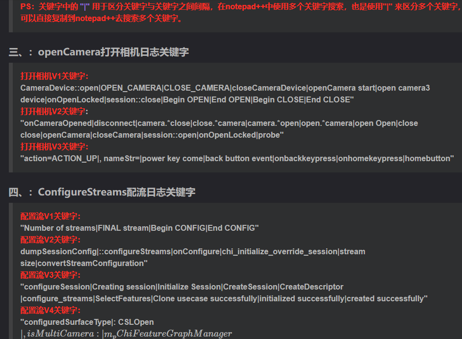
相机Camera日志实例分析之二:相机Camx【专业模式开启直方图拍照】单帧流程日志详解
【关注我,后续持续新增专题博文,谢谢!!!】 上一篇我们讲了: 这一篇我们开始讲: 目录 一、场景操作步骤 二、日志基础关键字分级如下 三、场景日志如下: 一、场景操作步骤 操作步…...

鱼香ros docker配置镜像报错:https://registry-1.docker.io/v2/
使用鱼香ros一件安装docker时的https://registry-1.docker.io/v2/问题 一键安装指令 wget http://fishros.com/install -O fishros && . fishros出现问题:docker pull 失败 网络不同,需要使用镜像源 按照如下步骤操作 sudo vi /etc/docker/dae…...
)
OpenLayers 分屏对比(地图联动)
注:当前使用的是 ol 5.3.0 版本,天地图使用的key请到天地图官网申请,并替换为自己的key 地图分屏对比在WebGIS开发中是很常见的功能,和卷帘图层不一样的是,分屏对比是在各个地图中添加相同或者不同的图层进行对比查看。…...
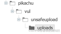
Unsafe Fileupload篇补充-木马的详细教程与木马分享(中国蚁剑方式)
在之前的皮卡丘靶场第九期Unsafe Fileupload篇中我们学习了木马的原理并且学了一个简单的木马文件 本期内容是为了更好的为大家解释木马(服务器方面的)的原理,连接,以及各种木马及连接工具的分享 文件木马:https://w…...
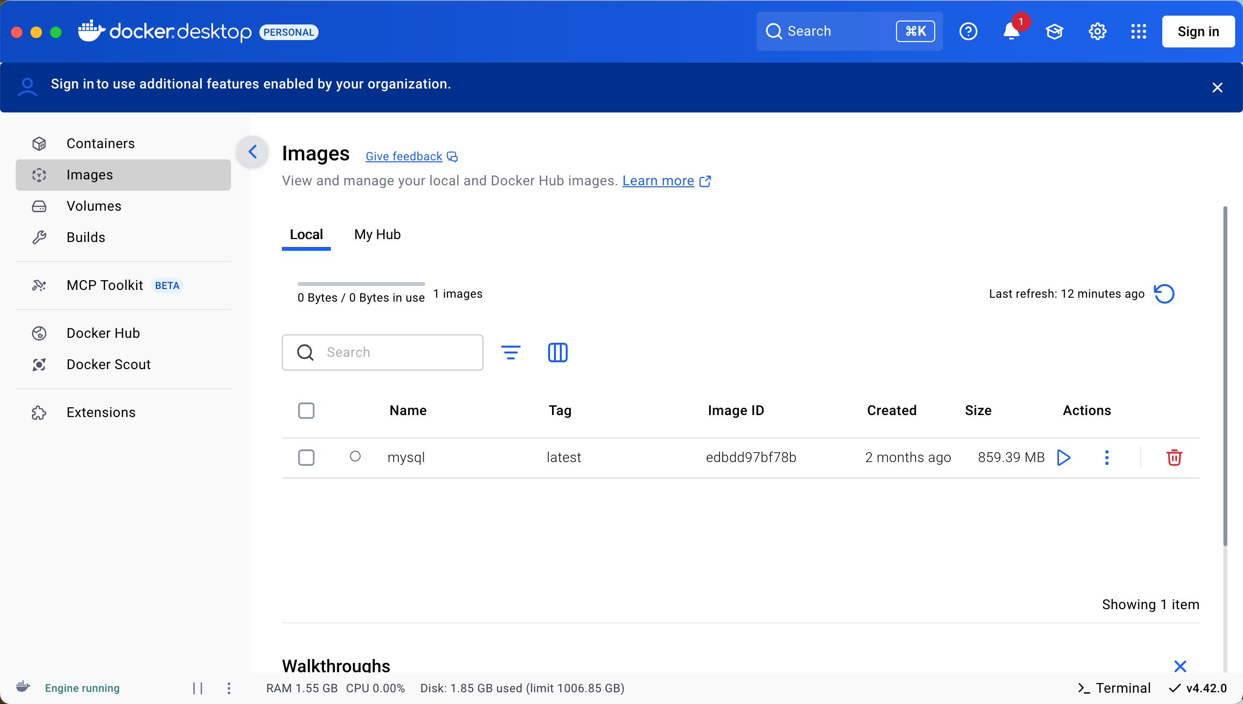
Docker 本地安装 mysql 数据库
Docker: Accelerated Container Application Development 下载对应操作系统版本的 docker ;并安装。 基础操作不再赘述。 打开 macOS 终端,开始 docker 安装mysql之旅 第一步 docker search mysql 》〉docker search mysql NAME DE…...

Git常用命令完全指南:从入门到精通
Git常用命令完全指南:从入门到精通 一、基础配置命令 1. 用户信息配置 # 设置全局用户名 git config --global user.name "你的名字"# 设置全局邮箱 git config --global user.email "你的邮箱example.com"# 查看所有配置 git config --list…...
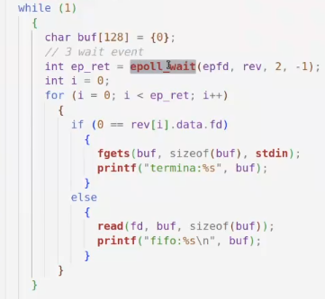
day36-多路IO复用
一、基本概念 (服务器多客户端模型) 定义:单线程或单进程同时监测若干个文件描述符是否可以执行IO操作的能力 作用:应用程序通常需要处理来自多条事件流中的事件,比如我现在用的电脑,需要同时处理键盘鼠标…...

android13 app的触摸问题定位分析流程
一、知识点 一般来说,触摸问题都是app层面出问题,我们可以在ViewRootImpl.java添加log的方式定位;如果是touchableRegion的计算问题,就会相对比较麻烦了,需要通过adb shell dumpsys input > input.log指令,且通过打印堆栈的方式,逐步定位问题,并找到修改方案。 问题…...

基于PHP的连锁酒店管理系统
有需要请加文章底部Q哦 可远程调试 基于PHP的连锁酒店管理系统 一 介绍 连锁酒店管理系统基于原生PHP开发,数据库mysql,前端bootstrap。系统角色分为用户和管理员。 技术栈 phpmysqlbootstrapphpstudyvscode 二 功能 用户 1 注册/登录/注销 2 个人中…...

探索Selenium:自动化测试的神奇钥匙
目录 一、Selenium 是什么1.1 定义与概念1.2 发展历程1.3 功能概述 二、Selenium 工作原理剖析2.1 架构组成2.2 工作流程2.3 通信机制 三、Selenium 的优势3.1 跨浏览器与平台支持3.2 丰富的语言支持3.3 强大的社区支持 四、Selenium 的应用场景4.1 Web 应用自动化测试4.2 数据…...