【阿旭机器学习实战】【35】员工离职率预测---决策树与随机森林预测
【阿旭机器学习实战】系列文章主要介绍机器学习的各种算法模型及其实战案例,欢迎点赞,关注共同学习交流。
本文的主要任务是通过决策树与随机森林模型预测一个员工离职的可能性并帮助人事部门理解员工为何离职。
目录
- 1.获取数据
- 2.数据预处理
- 3.分析数据
- 3.1 相关性分析
- 3.2 进行 T-Test
- 4. 建立预测模型:Decision Tree V.S. Random Forest
- 5. 模型评估
- 5.1ROC 图
- 5.2通过决策树分析不同的特征的重要性
1.获取数据
关注GZH:阿旭算法与机器学习,回复:“ML35”即可获取本文数据集、源码与项目文档
# 引入工具包
import pandas as pd
import numpy as np
import matplotlib.pyplot as plt
import matplotlib as matplot
import seaborn as sns
%matplotlib inline
# 读入数据到Pandas Dataframe "df"
df = pd.read_csv('HR_comma_sep.csv', index_col=None)
2.数据预处理
# 检测是否有缺失数据
df.isnull().any()
satisfaction_level       False
last_evaluation          False
number_project           False
average_montly_hours     False
time_spend_company       False
Work_accident            False
left                     False
promotion_last_5years    False
sales                    False
salary                   False
dtype: bool
# 数据的样例
df.head()
| satisfaction_level | last_evaluation | number_project | average_montly_hours | time_spend_company | Work_accident | left | promotion_last_5years | sales | salary | |
|---|---|---|---|---|---|---|---|---|---|---|
| 0 | 0.38 | 0.53 | 2 | 157 | 3 | 0 | 1 | 0 | sales | low |
| 1 | 0.80 | 0.86 | 5 | 262 | 6 | 0 | 1 | 0 | sales | medium |
| 2 | 0.11 | 0.88 | 7 | 272 | 4 | 0 | 1 | 0 | sales | medium |
| 3 | 0.72 | 0.87 | 5 | 223 | 5 | 0 | 1 | 0 | sales | low |
| 4 | 0.37 | 0.52 | 2 | 159 | 3 | 0 | 1 | 0 | sales | low |
注:“turnover”列为标签:1表示离职,0表示不离职,其他列均为特征值
# 重命名
df = df.rename(columns={'satisfaction_level': 'satisfaction', 'last_evaluation': 'evaluation','number_project': 'projectCount','average_montly_hours': 'averageMonthlyHours','time_spend_company': 'yearsAtCompany','Work_accident': 'workAccident','promotion_last_5years': 'promotion','sales' : 'department','left' : 'turnover'})
# 将预测标签‘是否离职’放在第一列
front = df['turnover']
df.drop(labels=['turnover'], axis=1, inplace = True)
df.insert(0, 'turnover', front)
df.head()
| turnover | satisfaction | evaluation | projectCount | averageMonthlyHours | yearsAtCompany | workAccident | promotion | department | salary | |
|---|---|---|---|---|---|---|---|---|---|---|
| 0 | 1 | 0.38 | 0.53 | 2 | 157 | 3 | 0 | 0 | sales | low |
| 1 | 1 | 0.80 | 0.86 | 5 | 262 | 6 | 0 | 0 | sales | medium |
| 2 | 1 | 0.11 | 0.88 | 7 | 272 | 4 | 0 | 0 | sales | medium |
| 3 | 1 | 0.72 | 0.87 | 5 | 223 | 5 | 0 | 0 | sales | low |
| 4 | 1 | 0.37 | 0.52 | 2 | 159 | 3 | 0 | 0 | sales | low |
3.分析数据
- 14999 条数据, 每一条数据包含 10 个特征
- 总的离职率: 24%
- 平均满意度为 0.61
df.shape
(14999, 10)
# 特征数据类型.
df.dtypes
turnover                 int64
satisfaction           float64
evaluation             float64
projectCount             int64
averageMonthlyHours      int64
yearsAtCompany           int64
workAccident             int64
promotion                int64
department              object
salary                  object
dtype: object
turnover_rate = df.turnover.value_counts() / len(df)
turnover_rate
0    0.761917
1    0.238083
Name: turnover, dtype: float64
# 显示统计数据
df.describe()
| turnover | satisfaction | evaluation | projectCount | averageMonthlyHours | yearsAtCompany | workAccident | promotion | |
|---|---|---|---|---|---|---|---|---|
| count | 14999.000000 | 14999.000000 | 14999.000000 | 14999.000000 | 14999.000000 | 14999.000000 | 14999.000000 | 14999.000000 |
| mean | 0.238083 | 0.612834 | 0.716102 | 3.803054 | 201.050337 | 3.498233 | 0.144610 | 0.021268 |
| std | 0.425924 | 0.248631 | 0.171169 | 1.232592 | 49.943099 | 1.460136 | 0.351719 | 0.144281 |
| min | 0.000000 | 0.090000 | 0.360000 | 2.000000 | 96.000000 | 2.000000 | 0.000000 | 0.000000 |
| 25% | 0.000000 | 0.440000 | 0.560000 | 3.000000 | 156.000000 | 3.000000 | 0.000000 | 0.000000 |
| 50% | 0.000000 | 0.640000 | 0.720000 | 4.000000 | 200.000000 | 3.000000 | 0.000000 | 0.000000 |
| 75% | 0.000000 | 0.820000 | 0.870000 | 5.000000 | 245.000000 | 4.000000 | 0.000000 | 0.000000 |
| max | 1.000000 | 1.000000 | 1.000000 | 7.000000 | 310.000000 | 10.000000 | 1.000000 | 1.000000 |
# 分组的平均数据统计
turnover_Summary = df.groupby('turnover')
turnover_Summary.mean()
| satisfaction | evaluation | projectCount | averageMonthlyHours | yearsAtCompany | workAccident | promotion | |
|---|---|---|---|---|---|---|---|
| turnover | |||||||
| 0 | 0.666810 | 0.715473 | 3.786664 | 199.060203 | 3.380032 | 0.175009 | 0.026251 |
| 1 | 0.440098 | 0.718113 | 3.855503 | 207.419210 | 3.876505 | 0.047326 | 0.005321 |
3.1 相关性分析
# 相关性矩阵
corr = df.corr()
#corr = (corr)
sns.heatmap(corr, xticklabels=corr.columns.values,yticklabels=corr.columns.values)corr
| turnover | satisfaction | evaluation | projectCount | averageMonthlyHours | yearsAtCompany | workAccident | promotion | |
|---|---|---|---|---|---|---|---|---|
| turnover | 1.000000 | -0.388375 | 0.006567 | 0.023787 | 0.071287 | 0.144822 | -0.154622 | -0.061788 |
| satisfaction | -0.388375 | 1.000000 | 0.105021 | -0.142970 | -0.020048 | -0.100866 | 0.058697 | 0.025605 |
| evaluation | 0.006567 | 0.105021 | 1.000000 | 0.349333 | 0.339742 | 0.131591 | -0.007104 | -0.008684 |
| projectCount | 0.023787 | -0.142970 | 0.349333 | 1.000000 | 0.417211 | 0.196786 | -0.004741 | -0.006064 |
| averageMonthlyHours | 0.071287 | -0.020048 | 0.339742 | 0.417211 | 1.000000 | 0.127755 | -0.010143 | -0.003544 |
| yearsAtCompany | 0.144822 | -0.100866 | 0.131591 | 0.196786 | 0.127755 | 1.000000 | 0.002120 | 0.067433 |
| workAccident | -0.154622 | 0.058697 | -0.007104 | -0.004741 | -0.010143 | 0.002120 | 1.000000 | 0.039245 |
| promotion | -0.061788 | 0.025605 | -0.008684 | -0.006064 | -0.003544 | 0.067433 | 0.039245 | 1.000000 |
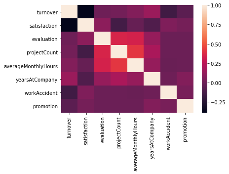
正相关的特征:
- projectCount VS evaluation: 0.349333
- projectCount VS averageMonthlyHours: 0.417211
- averageMonthlyHours VS evaluation: 0.339742
负相关的特征:
- satisfaction VS turnover: -0.388375
# 比较离职和未离职员工的满意度
emp_population = df['satisfaction'][df['turnover'] == 0].mean()
emp_turnover_satisfaction = df[df['turnover']==1]['satisfaction'].mean()print( '未离职员工满意度: ' + str(emp_population))
print( '离职员工满意度: ' + str(emp_turnover_satisfaction) )
未离职员工满意度: 0.666809590479516
离职员工满意度: 0.44009801176140917
3.2 进行 T-Test
进行一个 t-test, 看离职员工的满意度是不是和未离职员工的满意度明显不同
import scipy.stats as stats
stats.ttest_1samp(a = df[df['turnover']==1]['satisfaction'], # 离职员工的满意度样本popmean = emp_population)  # 未离职员工的满意度均值
Ttest_1sampResult(statistic=-51.3303486754725, pvalue=0.0)
T-Test 显示pvalue (0) 非常小, 所以他们之间是显著不同的
degree_freedom = len(df[df['turnover']==1])LQ = stats.t.ppf(0.025,degree_freedom)  # 95%致信区间的左边界RQ = stats.t.ppf(0.975,degree_freedom)  # 95%致信区间的右边界print ('The t-分布 左边界: ' + str(LQ))
print ('The t-分布 右边界: ' + str(RQ))
The t-分布 左边界: -1.9606285215955626
The t-分布 右边界: 1.9606285215955621
# 概率密度函数估计
fig = plt.figure(figsize=(15,4),)
ax=sns.kdeplot(df.loc[(df['turnover'] == 0),'evaluation'] , color='b',shade=True,label='no turnover')
ax=sns.kdeplot(df.loc[(df['turnover'] == 1),'evaluation'] , color='r',shade=True, label='turnover')
ax.set(xlabel='Employee Evaluation', ylabel='Frequency')
ax.legend()
plt.title('Employee Evaluation Distribution - Turnover V.S. No Turnover')
Text(0.5, 1.0, 'Employee Evaluation Distribution - Turnover V.S. No Turnover')

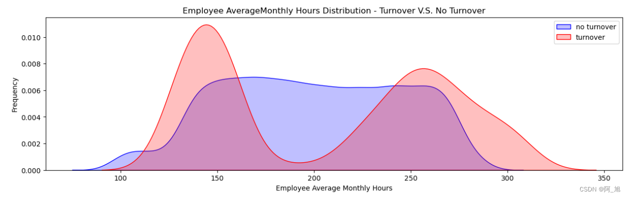
# 概率密度函数估计
fig = plt.figure(figsize=(15,4))
ax=sns.kdeplot(df.loc[(df['turnover'] == 0),'averageMonthlyHours'] , color='b',shade=True, label='no turnover')
ax=sns.kdeplot(df.loc[(df['turnover'] == 1),'averageMonthlyHours'] , color='r',shade=True, label='turnover')
ax.legend()
ax.set(xlabel='Employee Average Monthly Hours', ylabel='Frequency')
plt.title('Employee AverageMonthly Hours Distribution - Turnover V.S. No Turnover')
Text(0.5, 1.0, 'Employee AverageMonthly Hours Distribution - Turnover V.S. No Turnover')
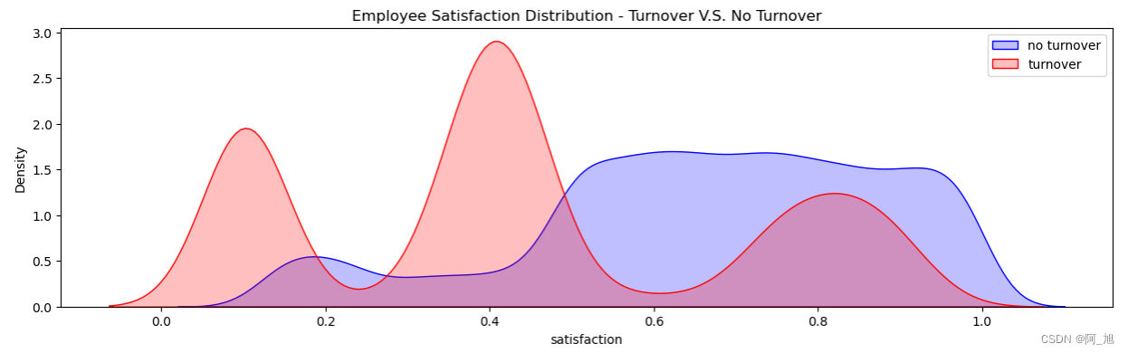
# 概率密度函数估计
fig = plt.figure(figsize=(15,4))
ax=sns.kdeplot(df.loc[(df['turnover'] == 0),'satisfaction'] , color='b',shade=True, label='no turnover')
ax=sns.kdeplot(df.loc[(df['turnover'] == 1),'satisfaction'] , color='r',shade=True, label='turnover')
plt.title('Employee Satisfaction Distribution - Turnover V.S. No Turnover')
ax.legend()
<matplotlib.legend.Legend at 0x281a5a6b820>
from sklearn.preprocessing import LabelEncoder
from sklearn.model_selection import train_test_split
from sklearn.metrics import accuracy_score, classification_report, precision_score, recall_score, confusion_matrix, precision_recall_curve
# 将string类型转换为整数类型
df["department"] = df["department"].astype('category').cat.codes
df["salary"] = df["salary"].astype('category').cat.codes# 产生X, y
target_name = 'turnover'
X = df.drop('turnover', axis=1)
y = df[target_name]# 将数据分为训练和测试数据集
# 注意参数 stratify = y 意味着在产生训练和测试数据中, 离职的员工的百分比等于原来总的数据中的离职的员工的百分比
X_train, X_test, y_train, y_test = train_test_split(X,y,test_size=0.15, random_state=123, stratify=y)df.head()
| turnover | satisfaction | evaluation | projectCount | averageMonthlyHours | yearsAtCompany | workAccident | promotion | department | salary | |
|---|---|---|---|---|---|---|---|---|---|---|
| 0 | 1 | 0.38 | 0.53 | 2 | 157 | 3 | 0 | 0 | 7 | 1 |
| 1 | 1 | 0.80 | 0.86 | 5 | 262 | 6 | 0 | 0 | 7 | 2 |
| 2 | 1 | 0.11 | 0.88 | 7 | 272 | 4 | 0 | 0 | 7 | 2 |
| 3 | 1 | 0.72 | 0.87 | 5 | 223 | 5 | 0 | 0 | 7 | 1 |
| 4 | 1 | 0.37 | 0.52 | 2 | 159 | 3 | 0 | 0 | 7 | 1 |
4. 建立预测模型:Decision Tree V.S. Random Forest
from sklearn.metrics import roc_auc_score
from sklearn.metrics import classification_report
from sklearn.ensemble import RandomForestClassifier
from sklearn import tree
from sklearn.tree import DecisionTreeClassifier# 决策树
dtree = tree.DecisionTreeClassifier(criterion='entropy',#max_depth=3, # 定义树的深度, 可以用来防止过拟合min_weight_fraction_leaf=0.01 # 定义叶子节点最少需要包含多少个样本(使用百分比表达), 防止过拟合)
dtree = dtree.fit(X_train,y_train)
print ("\n\n ---决策树---")
dt_roc_auc = roc_auc_score(y_test, dtree.predict(X_test))
print ("决策树 AUC = %2.2f" % dt_roc_auc)
print(classification_report(y_test, dtree.predict(X_test)))# 随机森林
rf = RandomForestClassifier(criterion='entropy',n_estimators=1000, max_depth=None, # 定义树的深度, 可以用来防止过拟合min_samples_split=10, # 定义至少多少个样本的情况下才继续分叉#min_weight_fraction_leaf=0.02 # 定义叶子节点最少需要包含多少个样本(使用百分比表达), 防止过拟合)
rf.fit(X_train, y_train)
print ("\n\n ---随机森林---")
rf_roc_auc = roc_auc_score(y_test, rf.predict(X_test))
print ("随机森林 AUC = %2.2f" % rf_roc_auc)
print(classification_report(y_test, rf.predict(X_test)))
 ---决策树---
决策树 AUC = 0.93precision    recall  f1-score   support0       0.97      0.98      0.97      17141       0.93      0.89      0.91       536accuracy                           0.96      2250macro avg       0.95      0.93      0.94      2250
weighted avg       0.96      0.96      0.96      2250---随机森林---
随机森林 AUC = 0.97precision    recall  f1-score   support0       0.98      1.00      0.99      17141       0.99      0.94      0.97       536accuracy                           0.98      2250macro avg       0.99      0.97      0.98      2250
weighted avg       0.98      0.98      0.98      2250
5. 模型评估
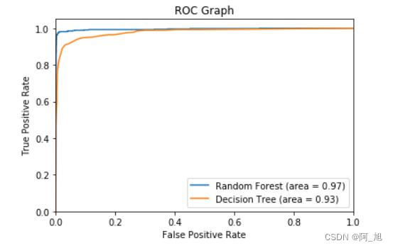
5.1ROC 图
# ROC 图
from sklearn.metrics import roc_curve
rf_fpr, rf_tpr, rf_thresholds = roc_curve(y_test, rf.predict_proba(X_test)[:,1])
dt_fpr, dt_tpr, dt_thresholds = roc_curve(y_test, dtree.predict_proba(X_test)[:,1])plt.figure()# 随机森林 ROC
plt.plot(rf_fpr, rf_tpr, label='Random Forest (area = %0.2f)' % rf_roc_auc)# 决策树 ROC
plt.plot(dt_fpr, dt_tpr, label='Decision Tree (area = %0.2f)' % dt_roc_auc)plt.xlim([0.0, 1.0])
plt.ylim([0.0, 1.05])
plt.xlabel('False Positive Rate')
plt.ylabel('True Positive Rate')
plt.title('ROC Graph')
plt.legend(loc="lower right")
plt.show()
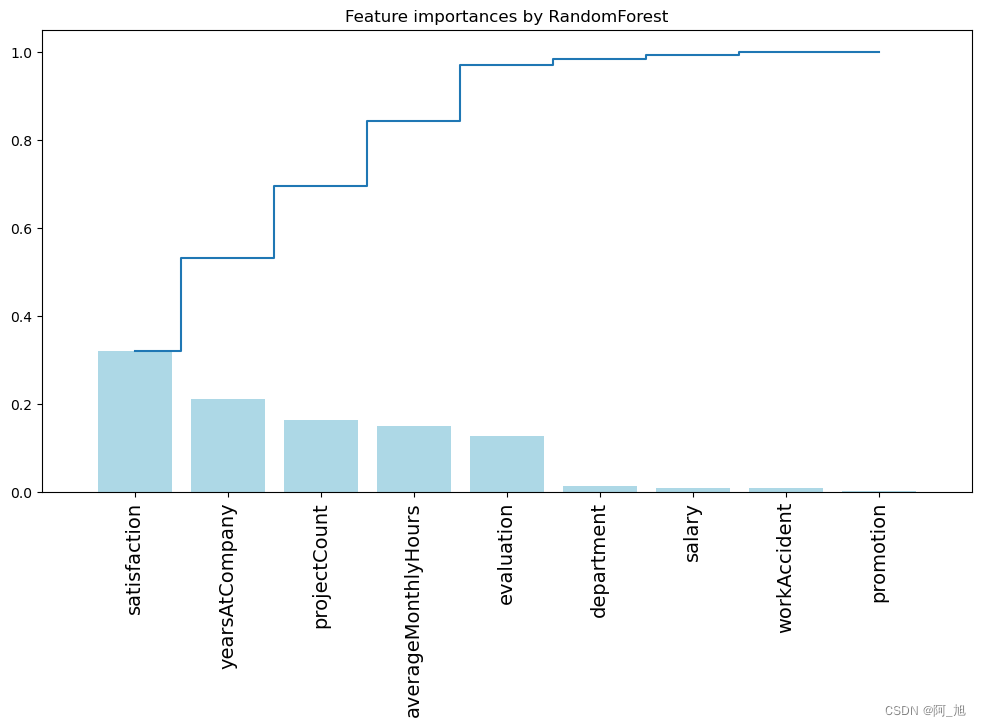
5.2通过决策树分析不同的特征的重要性
## 画出决策树特征的重要性 ##
importances = rf.feature_importances_
feat_names = df.drop(['turnover'],axis=1).columnsindices = np.argsort(importances)[::-1]
plt.figure(figsize=(12,6))
plt.title("Feature importances by RandomForest")
plt.bar(range(len(indices)), importances[indices], color='lightblue',  align="center")
plt.step(range(len(indices)), np.cumsum(importances[indices]), where='mid', label='Cumulative')
plt.xticks(range(len(indices)), feat_names[indices], rotation='vertical',fontsize=14)
plt.xlim([-1, len(indices)])
plt.show()
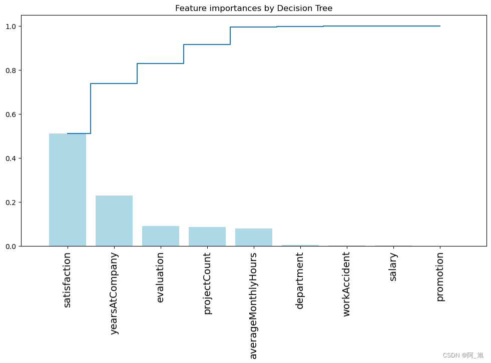
## 画出决策树的特征的重要性 ##
importances = dtree.feature_importances_
feat_names = df.drop(['turnover'],axis=1).columnsindices = np.argsort(importances)[::-1]
plt.figure(figsize=(12,6))
plt.title("Feature importances by Decision Tree")
plt.bar(range(len(indices)), importances[indices], color='lightblue',  align="center")
plt.step(range(len(indices)), np.cumsum(importances[indices]), where='mid', label='Cumulative')
plt.xticks(range(len(indices)), feat_names[indices], rotation='vertical',fontsize=14)
plt.xlim([-1, len(indices)])
plt.show()
如果文章对你有帮助,感谢点赞+关注!
关注下方GZH:阿旭算法与机器学习,回复:“ML35”即可获取本文数据集、源码与项目文档,欢迎共同学习交流
相关文章:
【阿旭机器学习实战】【35】员工离职率预测---决策树与随机森林预测
【阿旭机器学习实战】系列文章主要介绍机器学习的各种算法模型及其实战案例,欢迎点赞,关注共同学习交流。 本文的主要任务是通过决策树与随机森林模型预测一个员工离职的可能性并帮助人事部门理解员工为何离职。 目录1.获取数据2.数据预处理3.分析数据3.…...

Python学习-----模块4.0(json字符串与json模块)
目录 1.json简介: 2.json对象 3.json模块 (1)json.dumps() 函数 (2)json.dumps() 函数 (3)json.loads() 函数 (4) json.load() 函数 4.总结: 1.json简介: SON(…...

open3d最大平面检测,平面分割
1.点云读入 读入文件(配套点云下载链接) # 读取点云 pcd o3d.io.read_point_cloud("point_cloud_00000.ply")配套点云颜色为白色,open3d的点云显示默认背景为白色,所以将点云颜色更改为黑色 pcd.colors o3d.utilit…...
)
【C++】4.类和对象(下)
1.再谈构造函数 1赋值 class Date { public:Date(int year, int month, int day){_year year;_month month;_day day;}private:int _year;int _month;int _day; };构造函数体中的语句只能将其称作为赋初值,而不能称作初始化。因为初始化只能初始化一次…...
自动驾驶仿真:ECU TEST 、VTD、VERISTAND连接配置
文章目录一、ECU TEST 连接配置简介二、TBC配置 test bench configuration三、TCF配置 test configuration提示:以下是本篇文章正文内容,下面案例可供参考 一、ECU TEST 连接配置简介 1、ECU TEST(简称ET),用于HIL仿…...

postgres数据库连接管理
1.连接命令psql -d postgres -h 10.0.0.51. -p 1921 -U postgres(-d指定数据库名字)2.pg防火墙介绍(pg实例层面的权限控制)pg_hba.conf文件配置文件分为5部分:配置示例#TYPE DATABASE USER ADDRESS METHODhost all loc…...

【华为OD机试模拟题】用 C++ 实现 - 环中最长子串(2023.Q1)
最近更新的博客 华为OD机试 - 入栈出栈(C++) | 附带编码思路 【2023】 华为OD机试 - 箱子之形摆放(C++) | 附带编码思路 【2023】 华为OD机试 - 简易内存池 2(C++) | 附带编码思路 【2023】 华为OD机试 - 第 N 个排列(C++) | 附带编码思路 【2023】 华为OD机试 - 考古…...

Spring:@Async 注解和AsyncResult与CompletableFuture使用
Async概述 Spring中用Async注解标记的方法,称为异步方法,它会在调用方的当前线程之外的独立的线程中执行, 其实就相当于我们自己new Thread(()-> System.out.println("hello world !"))这样在另一个线程中去执行相应的业务逻辑…...

tidb ptca,ptcp考证
PingCAP 认证 TiDB 数据库专员 V6 考试(2023-02-23)https://learn.pingcap.com/learner/exam-market/list?categoryPCTA PingCAP 认证 TiDB 数据库管理专家(PCTP - DBA)认证考试范围指引 - ☄️ 学习与认证 - TiDB 的问答社区:lo…...
关于用windows开发遇到的各种乌龙事件之node版本管理---nvm install node之后 npm 找不到的问题
友情提醒,开发最好用nvm控制node版本 nrm 控制镜像源,能少掉很多头发开发过程中技术迭代更新的时候最要老命的就是 历史项目的node版本没有记录,导致开启旧项目的时候就会报错。尤其是npm 升级到8.x.x以后,各种版本不兼容。 真…...
JMeter做UI自动化
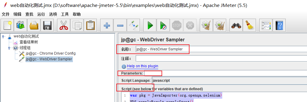
插件安装搜插件selenium,安装添加config添加线程组右键线程组->添加->配置元件->jpgc - Chrome Driver Configoption和proxy不解释了添加Sampler右键线程组->添加->取样器->jpgc - WebDriver Samplerscript language 选择:JavaScript&…...
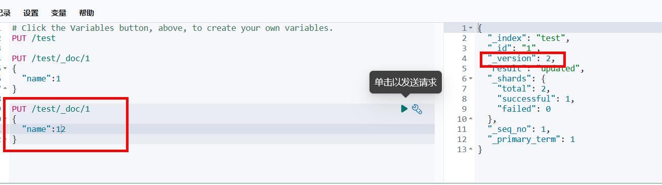
Kibana与Elasticsearch
下载与安装Kibanahttps://www.elastic.co/cn/downloads/kibanaKibana的版本与Elasticsearch的版本是一致的,使用方法也和Elasticsearch一致。由于我的英文不是特别好,我们找到config/kibana.yml末尾添加i18n.locale: "zh-CN" ,汉化…...
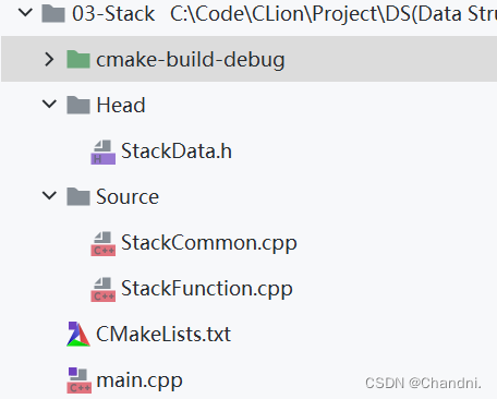
[数据结构]:03-栈(C语言实现)
目录 前言 已完成内容 单链表实现 01-开发环境 02-文件布局 03-代码 01-主函数 02-头文件 03-StackCommon.cpp 04-StackFunction.cpp 结语 前言 此专栏包含408考研数据结构全部内容,除其中使用到C引用外,全为C语言代码。使用C引用主要是为了简…...

1W+企业都在用的数字化管理秘籍,快收藏!
企业数字化,绕不开的话题。 随着国家相继出台各种举措助力中小企业数字化转型,积极推动产业数字化转型,培育数字经济新生态,企业想要谋生存,求发展,必然需要做好数字化转型和管理。 本篇文章想跟大家一起…...
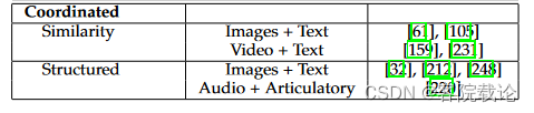
多模态机器学习入门——文献阅读(一)Multimodal Machine Learning: A Survey and Taxonomy
文章目录说明论文阅读AbstractIntroductionIntroduction总结Applications:A Historical Perspective补充与总结3 MULTIMODAL REPRESENTATIONS总结Joint Repersentations(1)总结和附加(一)Joint Repersentations(2)总结…...
)
通过哲学家进餐问题学习线程间协作(代码实现以leetcode1226为例)
哲学家进餐问题(代码实现以leetcode1226为例)问题场景解决思路解决死锁问题代码实现cgo(代码实现以leetcode1226为例) 提到多线程和锁解决问题,就想到了os中哲学家进餐问题。 问题场景 回想该问题产生场景,五个哲学家共用一张圆桌,分别坐在…...
消息队列--Kafka
Kafka简介集群部署配置Kafka测试Kafka1.Kafka简介 数据缓冲队列。同时提高了可扩展性。具有峰值处理能力,使用消息队列能够使关键组件顶住突发的访问压力,而不会因为突发的超负荷的请求而完全崩溃。 Kafka是一个分布式、支持分区的(partition…...

外盘国际期货:我国当代年轻人结婚逐年下降
我国当代年轻人 结婚现状结婚少了 结婚晚了 2013年后结婚人数逐年下降 结婚少了 离婚多了 结婚年龄越来越迟 以30岁为界线,30岁之后结婚占比逐年增加 2018 20-24岁:435.6万人 25-29岁:736.2万人 30-34岁:314.7万人 35-3…...

Ubuntu 22.04.2 发布,可更新至 Linux Kernel 5.19
Ubuntu 22.04 LTS (Jammy Jellyfish) Ubuntu 22.04.2 发布,可更新至 Linux Kernel 5.19 请访问原文链接:Ubuntu 22.04 LTS (Jammy Jellyfish),查看最新版。原创作品,转载请保留出处。 作者主页:www.sysin.org 发行说…...

论文阅读笔记——《室内服务机器人的实时场景分割算法》
一、主要工作 通过深度可分离卷积、膨胀卷积和通道注意力机制设计轻量级的高准确度特征提取模块。融合浅层特征与深层语义特征获得更丰富的图像特征。在NYUDv2和CamVid数据集上的MIoU分别达到72.7%和59.9%,模型的计算力为4.2GFLOPs,参数量为8.3Mb。 二…...
)
rknn优化教程(二)
文章目录 1. 前述2. 三方库的封装2.1 xrepo中的库2.2 xrepo之外的库2.2.1 opencv2.2.2 rknnrt2.2.3 spdlog 3. rknn_engine库 1. 前述 OK,开始写第二篇的内容了。这篇博客主要能写一下: 如何给一些三方库按照xmake方式进行封装,供调用如何按…...

.Net框架,除了EF还有很多很多......
文章目录 1. 引言2. Dapper2.1 概述与设计原理2.2 核心功能与代码示例基本查询多映射查询存储过程调用 2.3 性能优化原理2.4 适用场景 3. NHibernate3.1 概述与架构设计3.2 映射配置示例Fluent映射XML映射 3.3 查询示例HQL查询Criteria APILINQ提供程序 3.4 高级特性3.5 适用场…...

学校招生小程序源码介绍
基于ThinkPHPFastAdminUniApp开发的学校招生小程序源码,专为学校招生场景量身打造,功能实用且操作便捷。 从技术架构来看,ThinkPHP提供稳定可靠的后台服务,FastAdmin加速开发流程,UniApp则保障小程序在多端有良好的兼…...

反射获取方法和属性
Java反射获取方法 在Java中,反射(Reflection)是一种强大的机制,允许程序在运行时访问和操作类的内部属性和方法。通过反射,可以动态地创建对象、调用方法、改变属性值,这在很多Java框架中如Spring和Hiberna…...

【配置 YOLOX 用于按目录分类的图片数据集】
现在的图标点选越来越多,如何一步解决,采用 YOLOX 目标检测模式则可以轻松解决 要在 YOLOX 中使用按目录分类的图片数据集(每个目录代表一个类别,目录下是该类别的所有图片),你需要进行以下配置步骤&#x…...

Web 架构之 CDN 加速原理与落地实践
文章目录 一、思维导图二、正文内容(一)CDN 基础概念1. 定义2. 组成部分 (二)CDN 加速原理1. 请求路由2. 内容缓存3. 内容更新 (三)CDN 落地实践1. 选择 CDN 服务商2. 配置 CDN3. 集成到 Web 架构 …...

Java 二维码
Java 二维码 **技术:**谷歌 ZXing 实现 首先添加依赖 <!-- 二维码依赖 --><dependency><groupId>com.google.zxing</groupId><artifactId>core</artifactId><version>3.5.1</version></dependency><de…...
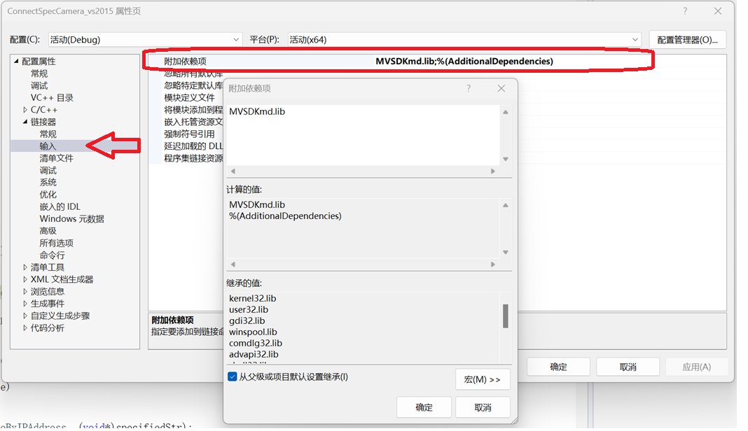
C/C++ 中附加包含目录、附加库目录与附加依赖项详解
在 C/C 编程的编译和链接过程中,附加包含目录、附加库目录和附加依赖项是三个至关重要的设置,它们相互配合,确保程序能够正确引用外部资源并顺利构建。虽然在学习过程中,这些概念容易让人混淆,但深入理解它们的作用和联…...
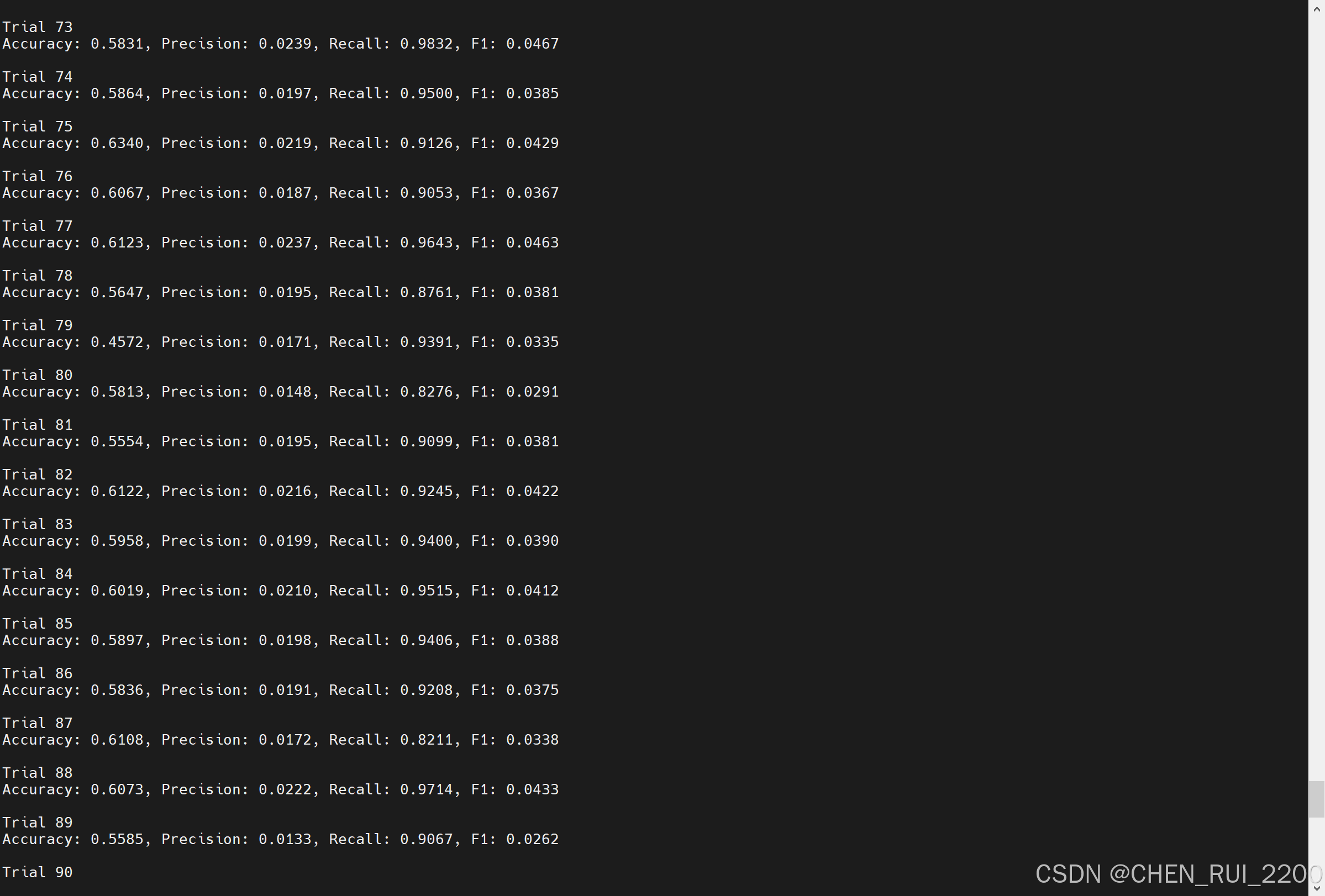
逻辑回归暴力训练预测金融欺诈
简述 「使用逻辑回归暴力预测金融欺诈,并不断增加特征维度持续测试」的做法,体现了一种逐步建模与迭代验证的实验思路,在金融欺诈检测中非常有价值,本文作为一篇回顾性记录了早年间公司给某行做反欺诈预测用到的技术和思路。百度…...

OD 算法题 B卷【正整数到Excel编号之间的转换】
文章目录 正整数到Excel编号之间的转换 正整数到Excel编号之间的转换 excel的列编号是这样的:a b c … z aa ab ac… az ba bb bc…yz za zb zc …zz aaa aab aac…; 分别代表以下的编号1 2 3 … 26 27 28 29… 52 53 54 55… 676 677 678 679 … 702 703 704 705;…...