Pytorch实现图片异常检测
图片异常检测
异常检测指的是在正常的图片中找到异常的数据,由于无法通过规则进行识别判断,这样的应用场景通常都是需要人工进行识别,比如残次品的识别,图片异常识别模型的目标是可以代替或者辅助人工进行识别异常图片。
AnoGAN 模型
由于正常图片的数据量远大于异常图片,可能只有 1/100 的图片是异常图片,甚至更小。通过图片分类模型很难实现异常图片的识别,因为无法找到足够的异常数据进行训练。因此,只能通过正常图片去构建异常检测模型。如何通过正常的图片实现检测异常图片的模型,可以使用之前用的对抗网络,通过识别网络进行检测,图片是正常数据还是伪造数据。AnoGAN 模型是用于识别异常图片的模型,如果只用GAN 模型中的识别网络进行判别,效果并不好,所以 AnoGAN 网络不光依靠识别网络,生成网络在其中也发挥重要的作用。
对于AnoGAN,对于输入的数据,AnoGAN 网络首先会对图片生成噪声 Z。通过噪声 Z 输入生成网络生成可以被识别的图片,如果训练集中不存在这样的图片,例如异常图片,那么生成网络是无法生成的,这类图片就是异常图片。
噪声 Z 的生成方式,初始状态噪声是随机生成的,随后噪声通过网络生成图片,把生成的图片训练集作比较,比较的方式是通过像素差值的绝对值求和,最后算出损失值,最后通过网络进行训练以减少损失值。
上述的这种损失值在AutoGen 中被称为 Residual Loss,如果只有 Residual Loss,模型效果有限。所以,AnoGAN 这里也利用了判别网络,将测试图像和生成图像输入到判别网络,并对判别网络的输出特征进行差值计算,这个差值称为 Discrimination loss。最后通过 Discrimination Loss 和 Residual Loss 合并组成损失函数。
数据准备
import os
import urllib.request
import zipfile
import tarfileimport matplotlib.pyplot as plt
%matplotlib inline
from PIL import Image
import numpy as np#不存在“data”文件夹时创建
data_dir = "./data/"
if not os.path.exists(data_dir):os.mkdir(data_dir)import sklearn
# 下载并读取MNIST的手写数字图像。
from sklearn.datasets import fetch_openmlmnist = fetch_openml('mnist_784', version=1, data_home="./data/")  #data_home指定保存地址。# 数据的提取
X = mnist.data
y = mnist.target# 将MNIST的第一个数据可视化
plt.imshow(np.array(X.iloc[0]).reshape(28, 28), cmap='gray')
print("这个图像数据的标签是{}".format(y[0]))#在文件夹“data”下创建文件夹“img_78”
data_dir_path = "./data/img_78/"
if not os.path.exists(data_dir_path):os.mkdir(data_dir_path)#从MNIST将数字7、8的图像作为图像保存到“img_78”文件夹中
count7=0
count8=0
max_num=200  # 每制作200张图片for i in range(len(X)):# 图像7的制作if (y[i] == "7") and (count7<max_num):file_path="./data/img_78/img_7_"+str(count7)+".jpg"im_f=(np.array(X.iloc[i]).reshape(28, 28))  # 将图像变形为28×28pil_img_f = Image.fromarray(im_f.astype(np.uint8))  # 把图像变成PILpil_img_f = pil_img_f.resize((64, 64), Image.BICUBIC)  # 扩大到64×64pil_img_f.save(file_path)  # 保存count7+=1 #图像8的制作if (y[i] == "8") and (count8<max_num):file_path="./data/img_78/img_8_"+str(count8)+".jpg"im_f=(np.array(X.iloc[i]).reshape(28, 28))  # 将图像变形为28*28pil_img_f = Image.fromarray(im_f.astype(np.uint8))  # 把图像变成PILpil_img_f = pil_img_f.resize((64, 64), Image.BICUBIC)  # 扩大到64×64pil_img_f.save(file_path)  # 保存count8+=1# 制作200张7和8之后,breakif (count7>=max_num) and (count8>=max_num):break# 在文件夹“data”下面创建文件夹“test”
data_dir_path = "./data/test/"
if not os.path.exists(data_dir_path):os.mkdir(data_dir_path)# 在上述制作7,8图像时使用的index的最终值
i_start = i+1
print(i_start)# 从MNIST将数字7、8的图像作为图像保存到“img_78”文件夹中
count2=0
count7=0
count8=0
max_num=5  #每制作五张图片for i in range(i_start,len(X)):  # 从i_start开始#图像2的制作if (y[i] == "2") and (count2<max_num):file_path="./data/test/img_2_"+str(count2)+".jpg"im_f=(np.array(X.iloc[i]).reshape(28, 28))  # 将图像变形为28×28pil_img_f = Image.fromarray(im_f.astype(np.uint8))  # 把图像变成PILpil_img_f = pil_img_f.resize((64, 64), Image.BICUBIC)  # 扩大到64×64pil_img_f.save(file_path)  # 保存count2+=1# 图像7的制作if (y[i] == "7") and (count7<max_num):file_path="./data/test/img_7_"+str(count7)+".jpg"im_f=(np.array(X.iloc[i]).reshape(28, 28))  #将图像变形为28×28pil_img_f = Image.fromarray(im_f.astype(np.uint8))  # 把图像变成PILpil_img_f = pil_img_f.resize((64, 64), Image.BICUBIC)  # 6扩大到64×64pil_img_f.save(file_path)  # 保存count7+=1 # 图像8的制作if (y[i] == "8") and (count8<max_num):file_path="./data/test/img_8_"+str(count8)+".jpg"im_f=(np.array(X.iloc[i]).reshape(28, 28))  # 将图像变形为28*28pil_img_f = Image.fromarray(im_f.astype(np.uint8))  # 把图像变成PILpil_img_f = pil_img_f.resize((64, 64), Image.BICUBIC)  # 扩大到64×64pil_img_f.save(file_path)  # 保存count8+=1 # 在文件夹“data”下创建文件夹“img_78_28size”
data_dir_path = "./data/img_78_28size/"
if not os.path.exists(data_dir_path):os.mkdir(data_dir_path)# 从MNIST将数字7、8的图像作为图像保存到“img_78_28size”文件夹中
count7=0
count8=0
max_num=200  # 每制作200张图片for i in range(len(X)):# 图像7的制作if (y[i] == "7") and (count7<max_num):file_path="./data/img_78_28size/img_7_"+str(count7)+".jpg"im_f=(np.array(X.iloc[i]).reshape(28, 28))  # 将图像变形为28×28pil_img_f = Image.fromarray(im_f.astype(np.uint8))  # 把图像变成PILpil_img_f.save(file_path)  # 保存count7+=1 # 图像8的制作if (y[i] == "8") and (count8<max_num):file_path="./data/img_78_28size/img_8_"+str(count8)+".jpg"im_f=(np.array(X.iloc[i]).reshape(28, 28))  # 将图像变形为28*28pil_img_f = Image.fromarray(im_f.astype(np.uint8))  # 画像变成PILpil_img_f.save(file_path)  # 保存count8+=1if (count7>=max_num) and (count8>=max_num):break# 在文件夹“data”下面创建文件夹“test”
data_dir_path = "./data/test_28size/"
if not os.path.exists(data_dir_path):os.mkdir(data_dir_path)# 在上述制作7,8图像时使用的index的最终值
i_start = i+1
print(i_start)# 从MNIST将数字7、8的图像作为图像保存到“img_78”文件夹中
count2=0
count7=0
count8=0
max_num=5  # 每制作五张图片for i in range(i_start,len(X)):  #从i_start开始# 图像2的制作if (y[i] == "2") and (count2<max_num):file_path="./data/test_28size/img_2_"+str(count2)+".jpg"im_f=(np.array(X.iloc[i]).reshape(28, 28))  # 将图像变形为28×28pil_img_f = Image.fromarray(im_f.astype(np.uint8))  # 把图像变成PILpil_img_f.save(file_path)  # 保存count2+=1 # 画像7的制作if (y[i] == "7") and (count7<max_num):file_path="./data/test_28size/img_7_"+str(count7)+".jpg"im_f=(np.array(X.iloc[i]).reshape(28, 28))  # 将图像变形为28×28pil_img_f = Image.fromarray(im_f.astype(np.uint8))  # 把图像变成PILpil_img_f.save(file_path)  # 保存count7+=1 # 图像8的制作if (y[i] == "8") and (count8<max_num):file_path="./data/test_28size/img_8_"+str(count8)+".jpg"im_f=(np.array(X.iloc[i]).reshape(28, 28))  # 将图像变形为28*28pil_img_f = Image.fromarray(im_f.astype(np.uint8))  # 把图像变成PILpil_img_f.save(file_path)  # 保存count8+=1
AnoGAN 实现
AnoGAN 网络实现以及训练、验证
# 导入软件包
import random
import math
import time
import pandas as pd
import numpy as np
from PIL import Imageimport torch
import torch.utils.data as data
import torch.nn as nn
import torch.nn.functional as F
import torch.optim as optimfrom torchvision import transforms# Setup seeds
torch.manual_seed(1234)
np.random.seed(1234)
random.seed(1234)class Generator(nn.Module):def __init__(self, z_dim=20, image_size=64):super(Generator, self).__init__()self.layer1 = nn.Sequential(nn.ConvTranspose2d(z_dim, image_size * 8,kernel_size=4, stride=1),nn.BatchNorm2d(image_size * 8),nn.ReLU(inplace=True))self.layer2 = nn.Sequential(nn.ConvTranspose2d(image_size * 8, image_size * 4,kernel_size=4, stride=2, padding=1),nn.BatchNorm2d(image_size * 4),nn.ReLU(inplace=True))self.layer3 = nn.Sequential(nn.ConvTranspose2d(image_size * 4, image_size * 2,kernel_size=4, stride=2, padding=1),nn.BatchNorm2d(image_size * 2),nn.ReLU(inplace=True))self.layer4 = nn.Sequential(nn.ConvTranspose2d(image_size * 2, image_size,kernel_size=4, stride=2, padding=1),nn.BatchNorm2d(image_size),nn.ReLU(inplace=True))self.last = nn.Sequential(nn.ConvTranspose2d(image_size, 1, kernel_size=4,stride=2, padding=1),nn.Tanh())#注意 :由于是黑白图像,因此输出通道数量为1def forward(self, z):out = self.layer1(z)out = self.layer2(out)out = self.layer3(out)out = self.layer4(out)out = self.last(out)return out# 动作确认
import matplotlib.pyplot as plt
%matplotlib inlineG = Generator(z_dim=20, image_size=64)# 输入的随机数
input_z = torch.randn(1, 20)# 将张量尺寸变形为(1,20,1,1)
input_z = input_z.view(input_z.size(0), input_z.size(1), 1, 1)# 输出假图像
fake_images = G(input_z)img_transformed = fake_images[0][0].detach().numpy()
plt.imshow(img_transformed, 'gray')
plt.show()class Discriminator(nn.Module):def __init__(self, z_dim=20, image_size=64):super(Discriminator, self).__init__()self.layer1 = nn.Sequential(nn.Conv2d(1, image_size, kernel_size=4,stride=2, padding=1),nn.LeakyReLU(0.1, inplace=True))#注意 :由于是黑白图像,因此输出通道数量为1self.layer2 = nn.Sequential(nn.Conv2d(image_size, image_size*2, kernel_size=4,stride=2, padding=1),nn.LeakyReLU(0.1, inplace=True))self.layer3 = nn.Sequential(nn.Conv2d(image_size*2, image_size*4, kernel_size=4,stride=2, padding=1),nn.LeakyReLU(0.1, inplace=True))self.layer4 = nn.Sequential(nn.Conv2d(image_size*4, image_size*8, kernel_size=4,stride=2, padding=1),nn.LeakyReLU(0.1, inplace=True))self.last = nn.Conv2d(image_size*8, 1, kernel_size=4, stride=1)def forward(self, x):out = self.layer1(x)out = self.layer2(out)out = self.layer3(out)out = self.layer4(out)feature = out #最后将通道集中到一个特征量中feature = feature.view(feature.size()[0], -1) #转换为二维out = self.last(out)return out, feature# 确认程序执
D = Discriminator(z_dim=20, image_size=64)#生成伪造图像
input_z = torch.randn(1, 20)
input_z = input_z.view(input_z.size(0), input_z.size(1), 1, 1)
fake_images = G(input_z)#将伪造的图像输入判别器D中
d_out = D(fake_images)# 将输出值d_out乘以Sigmoid函数,将其转换成0~1的值
print(nn.Sigmoid()(d_out[0]))# feature
print(d_out[1].shape)def make_datapath_list():"""制作用于学习、验证的图像数据和标注数据的文件路径表。 """train_img_list = list() # 保存图像文件路径for img_idx in range(200):img_path = "./data/img_78/img_7_" + str(img_idx)+'.jpg'train_img_list.append(img_path)img_path = "./data/img_78/img_8_" + str(img_idx)+'.jpg'train_img_list.append(img_path)return train_img_listclass ImageTransform():"""图像的预处理类"""def __init__(self, mean, std):self.data_transform = transforms.Compose([transforms.ToTensor(),transforms.Normalize(mean, std)])def __call__(self, img):return self.data_transform(img)
class GAN_Img_Dataset(data.Dataset):"""图像的Dataset类。继承PyTorch的Dataset类"""def __init__(self, file_list, transform):self.file_list = file_listself.transform = transformdef __len__(self):'''返回图像的张数'''return len(self.file_list)def __getitem__(self, index):'''获取经过预处理后的图像的张量格式的数据'''img_path = self.file_list[index]img = Image.open(img_path) # [高][宽]黑白#图像的预处理img_transformed = self.transform(img)return img_transformed#创建DataLoader并确认操作#创建文件列表
train_img_list=make_datapath_list()# 创建Dataset
mean = (0.5,)
std = (0.5,)
train_dataset = GAN_Img_Dataset(file_list=train_img_list, transform=ImageTransform(mean, std))# 创建DataLoader
batch_size = 64train_dataloader = torch.utils.data.DataLoader(train_dataset, batch_size=batch_size, shuffle=True)#确认执行结果
batch_iterator = iter(train_dataloader) # 转换成迭代器
imges = next(batch_iterator) #取出位于第一位的元素
print(imges.size()) # torch.Size([64, 1, 64, 64])#网络的初始化
def weights_init(m):classname = m.__class__.__name__if classname.find('Conv') != -1:#Conv2d和ConvTranspose2d的初始化nn.init.normal_(m.weight.data, 0.0, 0.02)nn.init.constant_(m.bias.data, 0)elif classname.find('BatchNorm') != -1:# BatchNorm2d的初始化nn.init.normal_(m.weight.data, 1.0, 0.02)nn.init.constant_(m.bias.data, 0)# 初始化的实施
G.apply(weights_init)
D.apply(weights_init)print("网络已经成功地完成了初始化")# 创建一个函数来学习模型def train_model(G, D, dataloader, num_epochs):#确认是否可以使用GPUdevice = torch.device("cuda:0" if torch.cuda.is_available() else "cpu")print("使用设备:", device)# 优化方法的设定g_lr, d_lr = 0.0001, 0.0004beta1, beta2 = 0.0, 0.9g_optimizer = torch.optim.Adam(G.parameters(), g_lr, [beta1, beta2])d_optimizer = torch.optim.Adam(D.parameters(), d_lr, [beta1, beta2])# 定义误差函数criterion = nn.BCEWithLogitsLoss(reduction='mean')# 使用硬编码的参数z_dim = 20mini_batch_size = 64#将网络变成GPUG.to(device)D.to(device)G.train() # 将模型转换为训练模式D.train() # 将模型转换为训练模式#如果网络相对固定,则开启加速torch.backends.cudnn.benchmark = True# 图像的张数num_train_imgs = len(dataloader.dataset)batch_size = dataloader.batch_size# 设置了迭代计数器iteration = 1logs = []#epoch循环for epoch in range(num_epochs):# 保存开始时间t_epoch_start = time.time()epoch_g_loss = 0.0 # epoch损失总和epoch_d_loss = 0.0 # epoch损失总和print('-------------')print('Epoch {}/{}'.format(epoch, num_epochs))print('-------------')print('(train)')# 以minibatch为单位从数据加载器中读取数据的循环for imges in dataloader:# --------------------# 1. 判别器D的学习# --------------------# 如果小批次的尺寸设置为1,会导致批次归一化处理产生错误,因此需要避免if imges.size()[0] == 1:continue#如果能使用GPU,则将数据送入GPU中imges = imges.to(device)#创建正确答案标签和伪造数据标签#在epoch最后的迭代中,小批次的数量会减少mini_batch_size = imges.size()[0]label_real = torch.full((mini_batch_size,), 1).to(device)label_fake = torch.full((mini_batch_size,), 0).to(device)#对真正的图像进行判定d_out_real, _ = D(imges)#生成伪造图像并进行判定input_z = torch.randn(mini_batch_size, z_dim).to(device)input_z = input_z.view(input_z.size(0), input_z.size(1), 1, 1)fake_images = G(input_z)d_out_fake, _ = D(fake_images)#计算误差d_loss_real = criterion(d_out_real.view(-1), label_real.float())d_loss_fake = criterion(d_out_fake.view(-1), label_fake.float())d_loss = d_loss_real + d_loss_fake#反向传播处理g_optimizer.zero_grad()d_optimizer.zero_grad()d_loss.backward()d_optimizer.step()# --------------------# 2.生成器G的学习# --------------------#生成伪造图像并进行判定input_z = torch.randn(mini_batch_size, z_dim).to(device)input_z = input_z.view(input_z.size(0), input_z.size(1), 1, 1)fake_images = G(input_z)d_out_fake, _ = D(fake_images)#计算误差g_loss = criterion(d_out_fake.view(-1), label_real.float())#反向传播处理g_optimizer.zero_grad()d_optimizer.zero_grad()g_loss.backward()g_optimizer.step()# --------------------# 3. 记录结果# --------------------epoch_d_loss += d_loss.item()epoch_g_loss += g_loss.item()iteration += 1#epoch的每个phase的loss和准确率t_epoch_finish = time.time()print('-------------')print('epoch {} || Epoch_D_Loss:{:.4f} ||Epoch_G_Loss:{:.4f}'.format(epoch, epoch_d_loss/batch_size, epoch_g_loss/batch_size))print('timer: {:.4f} sec.'.format(t_epoch_finish - t_epoch_start))t_epoch_start = time.time()print("总迭代次数:", iteration)return G, D# 进行训练和验证
num_epochs = 300
G_update, D_update = train_model(G, D, dataloader=train_dataloader, num_epochs=num_epochs)# 将生成图像和训练数据可视化device = torch.device("cuda:0" if torch.cuda.is_available() else "cpu")# 输入的随机数生成
batch_size = 8
z_dim = 20
fixed_z = torch.randn(batch_size, z_dim)
fixed_z = fixed_z.view(fixed_z.size(0), fixed_z.size(1), 1, 1)
fake_images = G_update(fixed_z.to(device))# 训练数据
batch_iterator = iter(train_dataloader) #转换成迭代器
imges = next(batch_iterator) #提取第1个要素#图像的可视化处理
fig = plt.figure(figsize=(15, 6))
for i in range(0, 5):#上层显示测试图像plt.subplot(2, 5, i+1)plt.imshow(imges[i][0].cpu().detach().numpy(), 'gray')#下层显示生成图像plt.subplot(2, 5, 5+i+1)plt.imshow(fake_images[i][0].cpu().detach().numpy(), 'gray')def Anomaly_score(x, fake_img, D, Lambda=0.1):#求测试图像x和生成图像fake_img的像素级差的绝对值,并对每个迷你批求和residual_loss = torch.abs(x-fake_img)residual_loss = residual_loss.view(residual_loss.size()[0], -1)residual_loss = torch.sum(residual_loss, dim=1)# 将测试图像x和生成图像fake_img输入到识别器D,取出特征量_, x_feature = D(x)_, G_feature = D(fake_img)# 求测试图像x和生成图像fake_img的特征量之差的绝对值,对每个迷你批次求和discrimination_loss = torch.abs(x_feature-G_feature)discrimination_loss = discrimination_loss.view(discrimination_loss.size()[0], -1)discrimination_loss = torch.sum(discrimination_loss, dim=1)# 将两种损失对每个迷你批进行加法运算loss_each = (1-Lambda)*residual_loss + Lambda*discrimination_loss#求迷你批的全部损失total_loss = torch.sum(loss_each)return total_loss, loss_each, residual_loss# 创建测试用的DataLoaderdef make_test_datapath_list():"""制作用于学习、验证的图像数据和标注数据的文件路径表。 """train_img_list = list() # 保存图像文件路径for img_idx in range(5):img_path = "./data/test/img_7_" + str(img_idx)+'.jpg'train_img_list.append(img_path)img_path = "./data/test/img_8_" + str(img_idx)+'.jpg'train_img_list.append(img_path)img_path = "./data/test/img_2_" + str(img_idx)+'.jpg'train_img_list.append(img_path)return train_img_list# 制作文件列表
test_img_list = make_test_datapath_list()# 制作Dataset
mean = (0.5,)
std = (0.5,)
test_dataset = GAN_Img_Dataset(file_list=test_img_list, transform=ImageTransform(mean, std))# 制作DataLoader
batch_size = 5test_dataloader = torch.utils.data.DataLoader(test_dataset, batch_size=batch_size, shuffle=False)# 测试数据的确认
batch_iterator = iter(test_dataloader) # 转换成迭代器
imges = next(batch_iterator) # 取出第一个迷你批次fig = plt.figure(figsize=(15, 6))
for i in range(0, 5):plt.subplot(2, 5, i+1)plt.imshow(imges[i][0].cpu().detach().numpy(), 'gray')# 想检测异常的图像
x = imges[0:5]
x = x.to(device)# 用于生成想要异常检测的图像的初始随机数
z = torch.randn(5, 20).to(device)
z = z.view(z.size(0), z.size(1), 1, 1)# 変将requires_grad设为True,使得变量z可以求导数
z.requires_grad = True#求z的优化函数,以便能够更新变量z
z_optimizer = torch.optim.Adam([z], lr=1e-3)#求z
for epoch in range(5000+1):fake_img = G_update(z)loss, _, _ = Anomaly_score(x, fake_img, D_update, Lambda=0.1)z_optimizer.zero_grad()loss.backward()z_optimizer.step()if epoch % 1000 == 0:print('epoch {} || loss_total:{:.0f} '.format(epoch, loss.item()))# 生成图像
fake_img = G_update(z)# 要求损失
loss, loss_each, residual_loss_each = Anomaly_score(x, fake_img, D_update, Lambda=0.1)#损失的计算总损失
loss_each = loss_each.cpu().detach().numpy()
print("total loss:", np.round(loss_each, 0))# 图像可视化
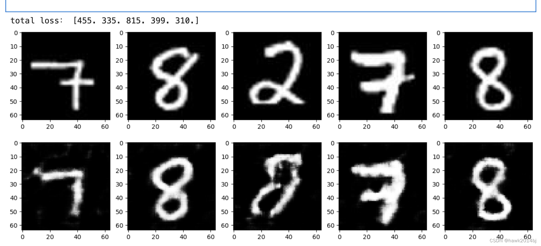
fig = plt.figure(figsize=(15, 6))
for i in range(0, 5):# 把测试数据放在上层plt.subplot(2, 5, i+1)plt.imshow(imges[i][0].cpu().detach().numpy(), 'gray')# 在下层显示生成数据plt.subplot(2, 5, 5+i+1)plt.imshow(fake_img[i][0].cpu().detach().numpy(), 'gray')可以看 2 的损失值最高,由此可判断 2 为异常图片。
Efficient GAN
AnoGAN 模型中,最重要的是 z 的取值,对z 的取值也有新的方法,其中一种就是 Efficient GAN,它优化了z 值的更新和学习时间。Efficient GAN是通过编码器的方式来对 z 值进行计算,Encoder通过 BiGAN 机制将图像于其关联在一起。
Efficient GAN 实现
通过 Efficient GAN 实现网络,并进行训练和验证。
# 导入软件包
import random
import math
import time
import pandas as pd
import numpy as np
from PIL import Imageimport torch
import torch.utils.data as data
import torch.nn as nn
import torch.nn.functional as F
import torch.optim as optimfrom torchvision import transforms# Setup seeds
torch.manual_seed(1234)
torch.cuda.manual_seed(1234)
np.random.seed(1234)
random.seed(1234)class Generator(nn.Module):def __init__(self, z_dim=20):super(Generator, self).__init__()self.layer1 = nn.Sequential(nn.Linear(z_dim, 1024),nn.BatchNorm1d(1024),nn.ReLU(inplace=True))self.layer2 = nn.Sequential(nn.Linear(1024, 7*7*128),nn.BatchNorm1d(7*7*128),nn.ReLU(inplace=True))self.layer3 = nn.Sequential(nn.ConvTranspose2d(in_channels=128, out_channels=64,kernel_size=4, stride=2, padding=1),nn.BatchNorm2d(64),nn.ReLU(inplace=True))self.last = nn.Sequential(nn.ConvTranspose2d(in_channels=64, out_channels=1,kernel_size=4, stride=2, padding=1),nn.Tanh())#注意 :由于是黑白图像,因此输出通道数量为 1def forward(self, z):out = self.layer1(z)out = self.layer2(out)#为了能置入卷积层中,需要对张量进行变形out = out.view(z.shape[0], 128, 7, 7)out = self.layer3(out)out = self.last(out)return out#确认执行结果
import matplotlib.pyplot as plt
%matplotlib inlineG = Generator(z_dim=20)
G.train()#输入的随机数
#由于要进行批次归一化处理,因此将小批次数设置为 2 以上
input_z = torch.randn(2, 20)#输出伪造图像
fake_images = G(input_z)  # torch.Size([2, 1, 28, 28])
img_transformed = fake_images[0][0].detach().numpy()
plt.imshow(img_transformed, 'gray')
plt.show()class Discriminator(nn.Module):def __init__(self, z_dim=20):super(Discriminator, self).__init__()#图像这边的输入处理self.x_layer1 = nn.Sequential(nn.Conv2d(1, 64, kernel_size=4,stride=2, padding=1),nn.LeakyReLU(0.1, inplace=True))#注意 :由于是黑白图像,因此输入通道数量为 1self.x_layer2 = nn.Sequential(nn.Conv2d(64, 64, kernel_size=4,stride=2, padding=1),nn.BatchNorm2d(64),nn.LeakyReLU(0.1, inplace=True))#随机数这边的输入处理self.z_layer1 = nn.Linear(z_dim, 512)#最终的判定self.last1 = nn.Sequential(nn.Linear(3648, 1024),nn.LeakyReLU(0.1, inplace=True))self.last2 = nn.Linear(1024, 1)def forward(self, x, z):#图像这边的输入处理x_out = self.x_layer1(x)x_out = self.x_layer2(x_out)#随机数这边的输入处理z = z.view(z.shape[0], -1)z_out = self.z_layer1(z)#将x_out与z_out连接在一起,交给全连接层进行判定x_out = x_out.view(-1, 64 * 7 * 7)out = torch.cat([x_out, z_out], dim=1)out = self.last1(out)feature = out  #最后将通道集中到一个特征量中feature = feature.view(feature.size()[0], -1)   #转换为二维out = self.last2(out)return out, feature#确认执行结果
D = Discriminator(z_dim=20)#生成伪造图像
input_z = torch.randn(2, 20)
fake_images = G(input_z)#将伪造图像输入判定器D中
d_out, _ = D(fake_images, input_z)#将输出结果d_out乘以Sigmoid,以将其转换为0~1的值
print(nn.Sigmoid()(d_out))class Encoder(nn.Module):def __init__(self, z_dim=20):super(Encoder, self).__init__()self.layer1 = nn.Sequential(nn.Conv2d(1, 32, kernel_size=3,stride=1),nn.LeakyReLU(0.1, inplace=True))#把图像转换成zself.layer2 = nn.Sequential(nn.Conv2d(32, 64, kernel_size=3,stride=2, padding=1),nn.BatchNorm2d(64),nn.LeakyReLU(0.1, inplace=True))self.layer3 = nn.Sequential(nn.Conv2d(64, 128, kernel_size=3,stride=2, padding=1),nn.BatchNorm2d(128),nn.LeakyReLU(0.1, inplace=True))#到这里为止,图像的尺寸为7像素×7像素self.last = nn.Linear(128 * 7 * 7, z_dim)def forward(self, x):out = self.layer1(x)out = self.layer2(out)out = self.layer3(out)#为了能放入FC中,对张量进行变形out = out.view(-1, 128 * 7 * 7)out = self.last(out)return out#确认执行结果
E = Encoder(z_dim=20)#输入的图像数据
x = fake_images  #fake_images是由上面的生成器G生成的#将图像编码为z
z = E(x)print(z.shape)
print(z)def make_datapath_list():"""制作用于学习、验证的图像数据和标注数据的文件路径表。 """train_img_list = list()  # 保存图像文件路径for img_idx in range(200):img_path = "./data/img_78_28size/img_7_" + str(img_idx)+'.jpg'train_img_list.append(img_path)img_path = "./data/img_78_28size/img_8_" + str(img_idx)+'.jpg'train_img_list.append(img_path)return train_img_listclass ImageTransform():"""图像的预处理类"""def __init__(self, mean, std):self.data_transform = transforms.Compose([transforms.ToTensor(),transforms.Normalize(mean, std)])def __call__(self, img):return self.data_transform(img)class GAN_Img_Dataset(data.Dataset):"""图像的Dataset类。继承PyTorch的Dataset类"""def __init__(self, file_list, transform):self.file_list = file_listself.transform = transformdef __len__(self):'''返回图像的张数'''return len(self.file_list)def __getitem__(self, index):'''获取预处理图像的Tensor格式数据'''img_path = self.file_list[index]img = Image.open(img_path)  # [高][宽]黑白# 图像的预处理img_transformed = self.transform(img)return img_transformed# 创建DataLoader并确认操作#制作文件列表
train_img_list=make_datapath_list()# Datasetを作成
mean = (0.5,)
std = (0.5,)
train_dataset = GAN_Img_Dataset(file_list=train_img_list, transform=ImageTransform(mean, std))# 制作DataLoader
batch_size = 64train_dataloader = torch.utils.data.DataLoader(train_dataset, batch_size=batch_size, shuffle=True)# 动作的确认
batch_iterator = iter(train_dataloader)  # 转换成迭代器
imges = next(batch_iterator)  # 找出第一个要素
print(imges.size())  # torch.Size([64, 1, 64, 64])#创建用于训练模型的函数def train_model(G, D, E, dataloader, num_epochs):#确认是否可以使用GPU加速device = torch.device("cuda:0" if torch.cuda.is_available() else "cpu")print("使用设备:", device)#设置最优化算法lr_ge = 0.0001lr_d = 0.0001/4beta1, beta2 = 0.5, 0.999g_optimizer = torch.optim.Adam(G.parameters(), lr_ge, [beta1, beta2])e_optimizer = torch.optim.Adam(E.parameters(), lr_ge, [beta1, beta2])d_optimizer = torch.optim.Adam(D.parameters(), lr_d, [beta1, beta2])#定义误差函数#BCEWithLogitsLoss是先将输入数据乘以Logistic,# 再计算二进制交叉熵criterion = nn.BCEWithLogitsLoss(reduction='mean')#对参数进行硬编码z_dim = 20mini_batch_size = 64#将网络载入GPU中G.to(device)E.to(device)D.to(device)G.train()  #将模型设置为训练模式E.train()  #将模型设置为训练模式D.train()  #将模型设置为训练模式#如果网络相对固定,则开启加速torch.backends.cudnn.benchmark = True#图像的张数num_train_imgs = len(dataloader.dataset)batch_size = dataloader.batch_size#设置迭代计数器iteration = 1logs = []# epoch循环for epoch in range(num_epochs):#保存开始时间t_epoch_start = time.time()epoch_g_loss = 0.0  #epoch的损失总和epoch_e_loss = 0.0  #epoch的损失总和epoch_d_loss = 0.0  #epoch的损失总和print('-------------')print('Epoch {}/{}'.format(epoch, num_epochs))print('-------------')print('(train)')#以minibatch为单位从数据加载器中读取数据的循环for imges in dataloader:#如果小批次的尺寸设置为1,会导致批次归一化处理产生错误,因此需要避免if imges.size()[0] == 1:continue#创建用于表示小批次尺寸为1和0的标签#创建正确答案标签和伪造数据标签#在epoch最后的迭代中,小批次的数量会减少mini_batch_size = imges.size()[0]label_real = torch.full((mini_batch_size,), 1).to(device)label_fake = torch.full((mini_batch_size,), 0).to(device)#如果能使用GPU,则将数据送入GPU中imges = imges.to(device)# --------------------# 1. 判别器D的学习# --------------------# 对真实的图像进行判定 z_out_real = E(imges)d_out_real, _ = D(imges, z_out_real)# 生成伪造图像并进行判定input_z = torch.randn(mini_batch_size, z_dim).to(device)fake_images = G(input_z)d_out_fake, _ = D(fake_images, input_z)#计算误差d_loss_real = criterion(d_out_real.view(-1), label_real.float())d_loss_fake = criterion(d_out_fake.view(-1), label_fake.float())d_loss = d_loss_real + d_loss_fake#反向传播d_optimizer.zero_grad()d_loss.backward()d_optimizer.step()# --------------------# 2. 生成器G的学习# --------------------#生成伪造图像并进行判定input_z = torch.randn(mini_batch_size, z_dim).to(device)fake_images = G(input_z)d_out_fake, _ = D(fake_images, input_z)#计算误差g_loss = criterion(d_out_fake.view(-1), label_real.float())#反向传播g_optimizer.zero_grad()g_loss.backward()g_optimizer.step()# --------------------# 3. 编码器E的学习# --------------------#对真实图像的z进行推定z_out_real = E(imges)d_out_real, _ = D(imges, z_out_real)#计算误差e_loss = criterion(d_out_real.view(-1), label_fake.float())#反向传播e_optimizer.zero_grad()e_loss.backward()e_optimizer.step()# --------------------#4.记录# --------------------epoch_d_loss += d_loss.item()epoch_g_loss += g_loss.item()epoch_e_loss += e_loss.item()iteration += 1#epoch的每个phase的loss和准确率t_epoch_finish = time.time()print('-------------')print('epoch {} || Epoch_D_Loss:{:.4f} ||Epoch_G_Loss:{:.4f} ||Epoch_E_Loss:{:.4f}'.format(epoch, epoch_d_loss/batch_size, epoch_g_loss/batch_size, epoch_e_loss/batch_size))print('timer:  {:.4f} sec.'.format(t_epoch_finish - t_epoch_start))t_epoch_start = time.time()print("总迭代次数:", iteration)return G, D, E#网络的初始化
def weights_init(m):classname = m.__class__.__name__if classname.find('Conv') != -1:#Conv2d和ConvTranspose2d的初始化nn.init.normal_(m.weight.data, 0.0, 0.02)nn.init.constant_(m.bias.data, 0)elif classname.find('BatchNorm') != -1:# BatchNorm2d的初始化nn.init.normal_(m.weight.data, 0.0, 0.02)nn.init.constant_(m.bias.data, 0)elif classname.find('Linear') != -1:#全连接层Linear的初始化m.bias.data.fill_(0)#开始初始化
G.apply(weights_init)
E.apply(weights_init)
D.apply(weights_init)print("网络已经成功地完成了初始化")# 进行训练和验证
num_epochs = 1500
G_update, D_update, E_update = train_model(G, D, E, dataloader=train_dataloader, num_epochs=num_epochs)#对生成图像与训练数据的可视化处理
device = torch.device("cuda:0" if torch.cuda.is_available() else "cpu")#生成输入的随机数
batch_size = 8
z_dim = 20
fixed_z = torch.randn(batch_size, z_dim)
fake_images = G_update(fixed_z.to(device))#训练数据
batch_iterator = iter(train_dataloader)  #转换成迭代器
imges = next(batch_iterator)  #取出最开头的元素#输出
fig = plt.figure(figsize=(15, 6))
for i in range(0, 5):#在上层中显示训练数据plt.subplot(2, 5, i+1)plt.imshow(imges[i][0].cpu().detach().numpy(), 'gray')#在下层中显示生成数据plt.subplot(2, 5, 5+i+1)plt.imshow(fake_images[i][0].cpu().detach().numpy(), 'gray')# ·制作测试用的Dataloaderdef make_test_datapath_list():"""制作用于学习、验证的图像数据和标注数据的文件路径表。 """train_img_list = list()  # ·保存图像文件路径for img_idx in range(5):img_path = "./data/test_28size/img_7_" + str(img_idx)+'.jpg'train_img_list.append(img_path)img_path = "./data/test_28size/img_8_" + str(img_idx)+'.jpg'train_img_list.append(img_path)img_path = "./data/test_28size/img_2_" + str(img_idx)+'.jpg'train_img_list.append(img_path)return train_img_list#制作文件列表
test_img_list = make_test_datapath_list()# 创建Dataset
mean = (0.5,)
std = (0.5,)
test_dataset = GAN_Img_Dataset(file_list=test_img_list, transform=ImageTransform(mean, std))# 制作DataLoader
batch_size = 5test_dataloader = torch.utils.data.DataLoader(test_dataset, batch_size=batch_size, shuffle=False)#训练数据
batch_iterator = iter(test_dataloader)  #转换成迭代器
imges = next(batch_iterator)  #取出最开头的元素fig = plt.figure(figsize=(15, 6))
for i in range(0, 5):#在下层中显示生成数据plt.subplot(2, 5, i+1)plt.imshow(imges[i][0].cpu().detach().numpy(), 'gray')def Anomaly_score(x, fake_img, z_out_real, D, Lambda=0.1):#计算测试图像x与生成图像fake_img在像素层次上的差值的绝对值,并以小批次为单位进行求和计算residual_loss = torch.abs(x-fake_img)residual_loss = residual_loss.view(residual_loss.size()[0], -1)residual_loss = torch.sum(residual_loss, dim=1)# 将测试图像x和生成图像fake_img输入判别器D中,并取出特征量图_, x_feature = D(x, z_out_real)_, G_feature = D(fake_img, z_out_real)# 计算测试图像x与生成图像fake_img的特征量的差的绝对值,并以小批次为单位进行求和计算discrimination_loss = torch.abs(x_feature-G_feature)discrimination_loss = discrimination_loss.view(discrimination_loss.size()[0], -1)discrimination_loss = torch.sum(discrimination_loss, dim=1)#将每个小批次中的两种损失相加loss_each = (1-Lambda)*residual_loss + Lambda*discrimination_loss#对所有批次中的损失进行计算total_loss = torch.sum(loss_each)return total_loss, loss_each, residual_loss#需要检测异常的图像
x = imges[0:5]
x = x.to(device)#对监督数据的图像进行编码,转换成z,再用生成器G生成图像
z_out_real = E_update(imges.to(device))
imges_reconstract = G_update(z_out_real)#计算损失值
loss, loss_each, residual_loss_each = Anomaly_score(x, imges_reconstract, z_out_real, D_update, Lambda=0.1)#计算损失值,损失总和
loss_each = loss_each.cpu().detach().numpy()
print("total loss:", np.round(loss_each, 0))#图像的可视化
fig = plt.figure(figsize=(15, 6))
for i in range(0, 5):#在上层中显示训练数据plt.subplot(2, 5, i+1)plt.imshow(imges[i][0].cpu().detach().numpy(), 'gray')#在下层中显示生成数据plt.subplot(2, 5, 5+i+1)plt.imshow(imges_reconstract[i][0].cpu().detach().numpy(), 'gray')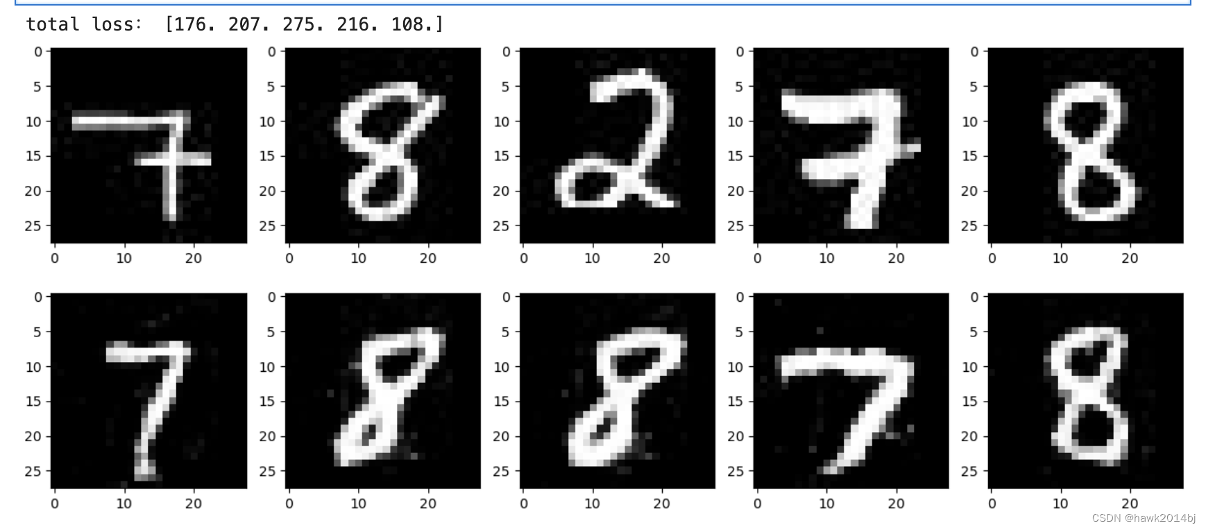
AnoGAN 模型可以进行异常图片的识别,这个例子比较简单,由于是单通道训练,随意模型训练比较快。如果是彩色图片,训练改时间会更久,在业务场景中可以调整阈值,例如Loss高于 250 为异常图片。
相关文章:
Pytorch实现图片异常检测
图片异常检测 异常检测指的是在正常的图片中找到异常的数据,由于无法通过规则进行识别判断,这样的应用场景通常都是需要人工进行识别,比如残次品的识别,图片异常识别模型的目标是可以代替或者辅助人工进行识别异常图片。 AnoGAN…...

【NOI-题解】1586. 扫地机器人1430 - 迷宫出口1434. 数池塘(四方向)1435. 数池塘(八方向)
文章目录 一、前言二、问题问题:1586 - 扫地机器人问题:1430 - 迷宫出口问题:1434. 数池塘(四方向)问题:1435. 数池塘(八方向) 三、感谢 一、前言 本章节主要对深搜基础题目进行讲解…...

探究MySQL行格式:解析DYNAMIC与COMPACT的异同
在MySQL中,行格式对于数据存储和检索起着至关重要的作用。MySQL提供了多种行格式,其中DYNAMIC和COMPACT是两种常见的行格式。 本文将深入探讨MySQL行格式DYNAMIC和COMPACT的区别,帮助读者更好地理解它们的特点和适用场景。 1. MySQL行格式简…...
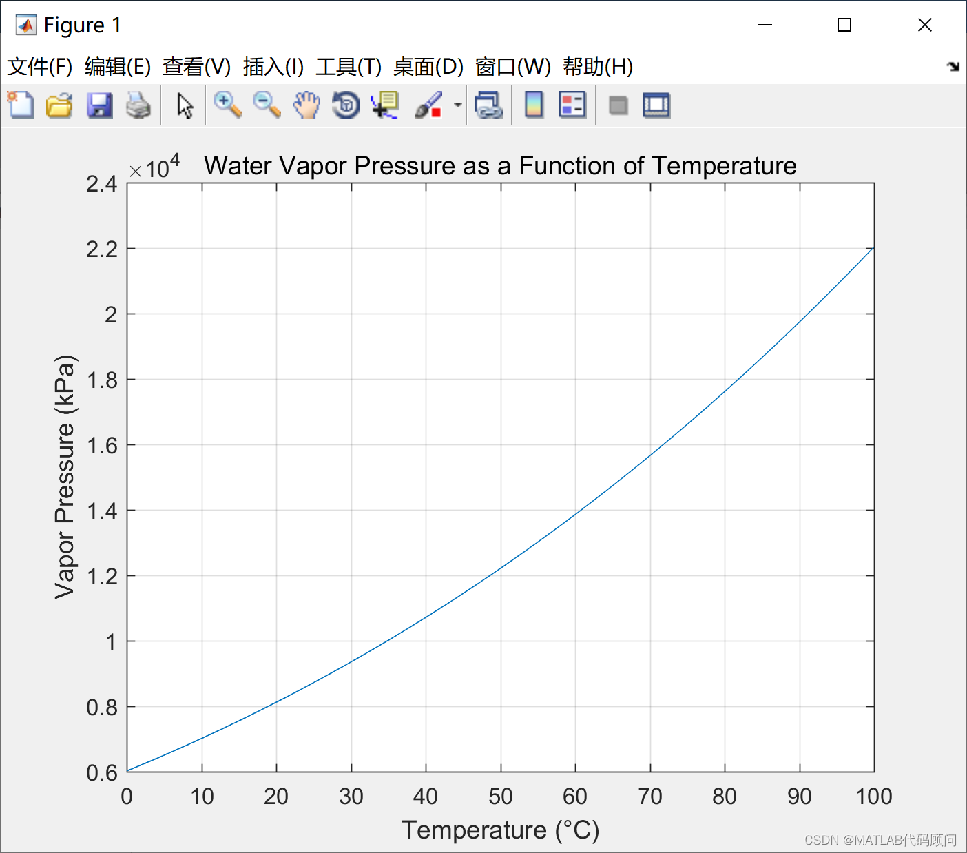
MATLAB绘制蒸汽压力和温度曲线
蒸汽压力与温度之间的具体关系公式一般采用安托因方程(Antoine Equation),用于描述纯物质的蒸汽压与温度之间的关系。安托因方程的一般形式如下: [\log_{10} P A - \frac{B}{C T}] 其中, (P) 是蒸汽压(…...
repo跟git的关系
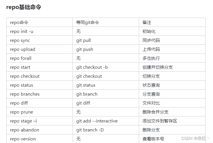
关于repo 大都讲的太复杂了,大多是从定义角度跟命令角度去讲解,其实从现实项目使用角度而言repo很好理解. 我们都知道git是用来管理项目的,多人开发过程中git功能很好用.现在我们知道一个项目会用一个git仓库去管理,项目的开发过程中会使用git创建分支之类的来更好的维护项目代…...
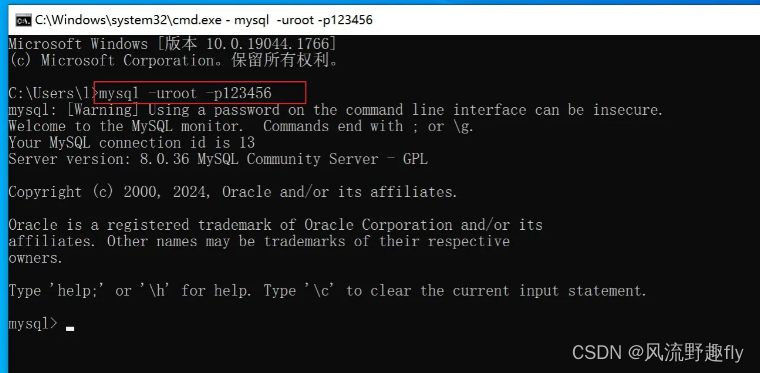
Mysql 8.0 -- 最新版本安装(保姆级教程)
Mysql 8.0 -- 最新版本安装(保姆级教程) 一,下载Mysql数据库: 官网链接:https://www.mysql.com/downloads/ 二,安装Mysql: 三,找到Mysql安装目录: 找到mysql安装目录…...
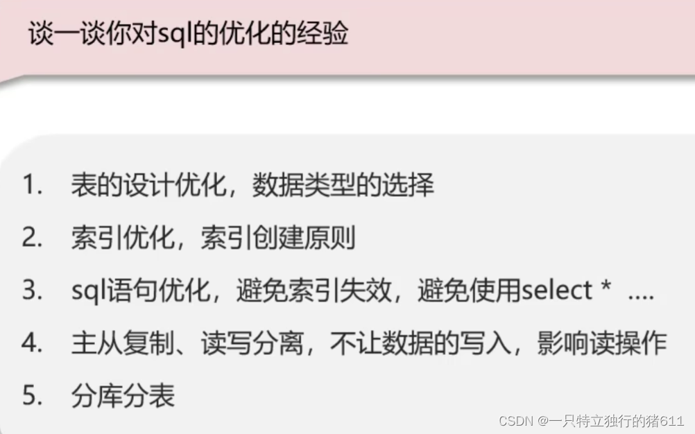
sql优化思路
sql的优化经验 这里解释一下SQL语句的优化的原理 1.指明字段名称,可以尽量使用覆盖索引,避免回表查询,因此可以提高效率 2.字面意思,无需过多赘述。索引就是为了提高查询效率的。 3.图中两条sql直接可以使用union all 或者 uni…...

gin学习1-7
package mainimport ("github.com/gin-gonic/gin""net/http" )// 响应json还有其他响应差不多可以去学 func _string(c *gin.Context) {c.String(http.StatusOK, "lalal") } func _json(c *gin.Context) {//json响应结构体type UsetInfo struct …...
likeshop多商户单商户商城_likeshop跑腿源码_likeshop物品租赁系统开源版怎么配置小程序对接?
本人是商业用户所以能持续得到最新商业版,今天我说下likeshop里面怎么打包小程序,大家得到程序时候会发现它有admin目录 app目录 server目录 这三个目录分别是做什么呢? 1.admin目录 下面都是架构文件使用得是Node.js打包得,至于…...
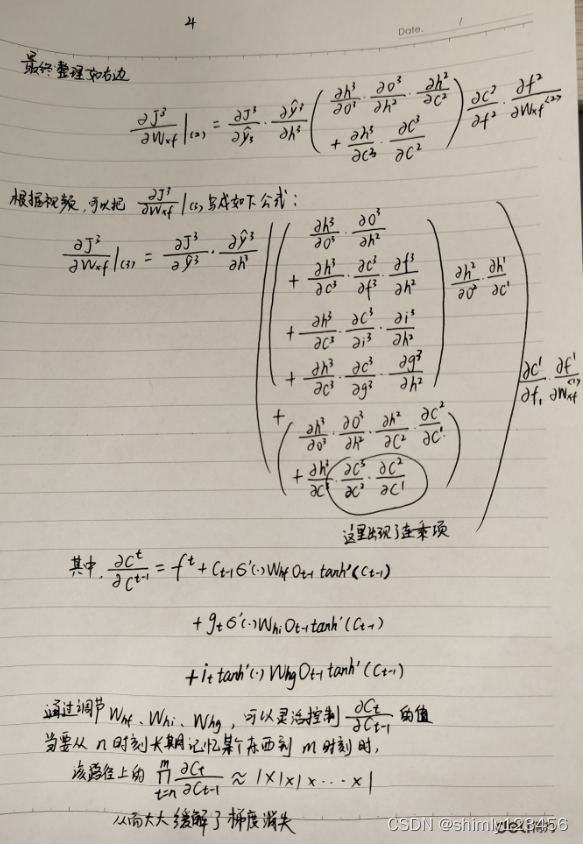
(done) LSTM 详解 (包括它为什么能缓解梯度消失)
RNN 参考视频:https://www.bilibili.com/video/BV1e5411K7oW/?p2&spm_id_frompageDriver&vd_source7a1a0bc74158c6993c7355c5490fc600 LSTM 参考视频:https://www.bilibili.com/video/BV1qM4y1M7Nv?p5&vd_source7a1a0bc74158c6993c7355c5…...
springboot使用研究
map-underscore-to-camel-case: true 开启驼峰命名 GetMapping("/userInfo")public Result<Users> userInfo(RequestHeader(name "Authorization") String token,HttpServletResponse response) {Map<String, Object> map JwtUtil.parseT…...
老旧房屋用电线路故障引起的电气火灾预防对策
摘 要:在我国新农村建设方针指引下,农村地区的发展水平有了显著提高。在农村经济发展中,我们也要认识到其中存在的风险隐患问题,其中重要的就是火灾事故。火灾事故给农村发展带来的不利影响,不仅严重威胁到农村群众的生…...
OpenAI发布GPT-4.0使用指南
大家好,ChatGPT 自诞生以来,凭借划时代的创新,被无数人一举送上生成式 AI 的神坛。在使用时,总是期望它能准确理解我们的意图,却时常发现其回答或创作并非百分之百贴合期待。这种落差可能源于我们对于模型性能的过高期…...

【WEEK11】学习目标及总结【Spring Boot】【中文版】
学习目标: 学习SpringBoot 学习内容: 参考视频教程【狂神说Java】SpringBoot最新教程IDEA版通俗易懂员工管理系统 页面国际化登录功能展示员工列表增加员工修改员工信息删除及404处理 学习时间及产出: 第十一周MON~SAT 2024.5.6【WEEK11】…...
Unity 性能优化之图片优化(八)
提示:仅供参考,有误之处,麻烦大佬指出,不胜感激! 文章目录 前言一、可以提前和美术商量的事1.避免内存浪费(UI图片,不是贴图)2.提升图片性能 二、图片优化1.图片Max Size修改&#x…...
C++类细节,面试题02
文章目录 2. 虚函数vs纯虚函数3. 重写vs重载vs隐藏3.1. 为什么C可以重载? 4. 类变量vs实例变量5. 类方法及其特点6. 空类vs空结构体6.1. 八个默认函数:6.2. 为什么空类占用1字节 7. const作用7.1 指针常量vs常量指针vs常量指针常量 8. 接口vs抽象类9. 浅…...

Stylus的引入
Stylus是一个CSS预处理器,它允许开发者使用更高级的语法来编写CSS,并提供了一些额外的功能来简化和增强CSS的编写过程。以下是关于Stylus的详解和引入方法的详细介绍: 一、Stylus的详解 特点和功能: 变量:允许你定义…...
前端框架-echarts
Echarts 项目中要使用到echarts框架,从零开始在csdn上记笔记。 这是一个基础的代码,小白入门看一下 <!DOCTYPE html> <html lang"en"> <head><meta charset"UTF-8"><meta name"viewport" co…...
【StarRocks系列】 Trino 方言支持
我们在之前的文章中,介绍了 Doris 官方提供的两种方言转换工具,分别是 sql convertor 和方言 plugin。StarRocks 目前同样也提供了类似的方言转换功能。本文我们就一起来看一下这个功能的实现与 Doris 相比有何不同。 一、Trino 方言验证 我们可以通过…...
【2024最新华为OD-C卷试题汇总】URL拼接 (100分) - 三语言AC题解(Python/Java/Cpp)
🍭 大家好这里是清隆学长 ,一枚热爱算法的程序员 ✨ 本系列打算持续跟新华为OD-C卷的三语言AC题解 💻 ACM银牌🥈| 多次AK大厂笔试 | 编程一对一辅导 👏 感谢大家的订阅➕ 和 喜欢💗 文章目录 前…...
: K8s 核心概念白话解读(上):Pod 和 Deployment 究竟是什么?)
云原生核心技术 (7/12): K8s 核心概念白话解读(上):Pod 和 Deployment 究竟是什么?
大家好,欢迎来到《云原生核心技术》系列的第七篇! 在上一篇,我们成功地使用 Minikube 或 kind 在自己的电脑上搭建起了一个迷你但功能完备的 Kubernetes 集群。现在,我们就像一个拥有了一块崭新数字土地的农场主,是时…...

C++初阶-list的底层
目录 1.std::list实现的所有代码 2.list的简单介绍 2.1实现list的类 2.2_list_iterator的实现 2.2.1_list_iterator实现的原因和好处 2.2.2_list_iterator实现 2.3_list_node的实现 2.3.1. 避免递归的模板依赖 2.3.2. 内存布局一致性 2.3.3. 类型安全的替代方案 2.3.…...

【磁盘】每天掌握一个Linux命令 - iostat
目录 【磁盘】每天掌握一个Linux命令 - iostat工具概述安装方式核心功能基础用法进阶操作实战案例面试题场景生产场景 注意事项 【磁盘】每天掌握一个Linux命令 - iostat 工具概述 iostat(I/O Statistics)是Linux系统下用于监视系统输入输出设备和CPU使…...
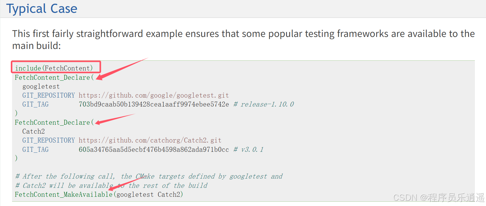
CMake 从 GitHub 下载第三方库并使用
有时我们希望直接使用 GitHub 上的开源库,而不想手动下载、编译和安装。 可以利用 CMake 提供的 FetchContent 模块来实现自动下载、构建和链接第三方库。 FetchContent 命令官方文档✅ 示例代码 我们将以 fmt 这个流行的格式化库为例,演示如何: 使用 FetchContent 从 GitH…...

今日科技热点速览
🔥 今日科技热点速览 🎮 任天堂Switch 2 正式发售 任天堂新一代游戏主机 Switch 2 今日正式上线发售,主打更强图形性能与沉浸式体验,支持多模态交互,受到全球玩家热捧 。 🤖 人工智能持续突破 DeepSeek-R1&…...

AirSim/Cosys-AirSim 游戏开发(四)外部固定位置监控相机
这个博客介绍了如何通过 settings.json 文件添加一个无人机外的 固定位置监控相机,因为在使用过程中发现 Airsim 对外部监控相机的描述模糊,而 Cosys-Airsim 在官方文档中没有提供外部监控相机设置,最后在源码示例中找到了,所以感…...
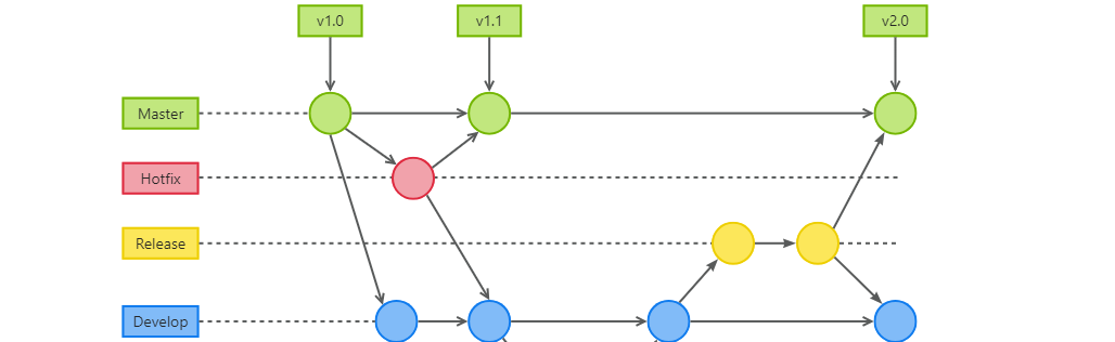
GitFlow 工作模式(详解)
今天再学项目的过程中遇到使用gitflow模式管理代码,因此进行学习并且发布关于gitflow的一些思考 Git与GitFlow模式 我们在写代码的时候通常会进行网上保存,无论是github还是gittee,都是一种基于git去保存代码的形式,这样保存代码…...
mac 安装homebrew (nvm 及git)
mac 安装nvm 及git 万恶之源 mac 安装这些东西离不开Xcode。及homebrew 一、先说安装git步骤 通用: 方法一:使用 Homebrew 安装 Git(推荐) 步骤如下:打开终端(Terminal.app) 1.安装 Homebrew…...

从 GreenPlum 到镜舟数据库:杭银消费金融湖仓一体转型实践
作者:吴岐诗,杭银消费金融大数据应用开发工程师 本文整理自杭银消费金融大数据应用开发工程师在StarRocks Summit Asia 2024的分享 引言:融合数据湖与数仓的创新之路 在数字金融时代,数据已成为金融机构的核心竞争力。杭银消费金…...

第7篇:中间件全链路监控与 SQL 性能分析实践
7.1 章节导读 在构建数据库中间件的过程中,可观测性 和 性能分析 是保障系统稳定性与可维护性的核心能力。 特别是在复杂分布式场景中,必须做到: 🔍 追踪每一条 SQL 的生命周期(从入口到数据库执行)&#…...